#——————————————————————————————————- #NEURONRAIN ASFER - Software for Mining Large Datasets #This program is free software: you can redistribute it and/or modify #it under the terms of the GNU General Public License as published by #the Free Software Foundation, either version 3 of the License, or #(at your option) any later version. #This program is distributed in the hope that it will be useful, #but WITHOUT ANY WARRANTY; without even the implied warranty of #MERCHANTABILITY or FITNESS FOR A PARTICULAR PURPOSE. See the #GNU General Public License for more details. #You should have received a copy of the GNU General Public License #along with this program. If not, see <http://www.gnu.org/licenses/>. #——————————————————————————————————– #K.Srinivasan #NeuronRain Documentation and Licensing: http://neuronrain-documentation.readthedocs.io/en/latest/ #Personal website(research): https://acadpdrafts.readthedocs.io/en/latest/ # (links to mirror of erstwhile https://sites.google.com/site/kuja27 and all references to it are redirected # implicitly to https://acadpdrafts.readthedocs.io/en/latest/) #——————————————————————————————————–
Document Licensed by:
<a rel=”license” href=”http://creativecommons.org/licenses/by-nc-nd/4.0/”><img alt=”Creative Commons Licence” style=”border-width:0” src=”https://i.creativecommons.org/l/by-nc-nd/4.0/88x31.png” /></a><br />This work is licensed under a <a rel=”license” href=”http://creativecommons.org/licenses/by-nc-nd/4.0/”>Creative Commons Attribution-NonCommercial-NoDerivatives 4.0 International License</a>.
NeuronRain - Design Objectives
NeuronRain OS is machine learning, cloud primitives enriched linux-kernel fork-off with applications in Internet-of-Things. AstroInfer is the machine learning side of it to learn analytics variables later read as config by linux kernel and any device specific driver. NeuronRain has been partitioned into components so that effective decoupling is achieved e.g Linux kernel can be realtime OS for realtime less-latency applications, Message Queuing can be KingCobra or any other standard MQ product. There are IOT operating systems like https://github.com/RIOT-OS/. Linux and IoT - linux on cameras,automobiles etc., - https://lwn.net/Articles/596754/. NeuronRain in itself is not just a product but a framework to build products. Applications can invoke VIRGO cloud memory,clone,filesystem primitives to create new products on NeuronRain Smart-IoT framework.
Copyright attributions for other open source products dependencies:
1.Maitreya’s Dreams - http://www.saravali.de (some bugs were fixed locally in degree computation of textual display mode) 2.SVMLight - http://svmlight.joachims.org/ 3.BioPython and ClustalOmega Multiple Sequence Alignment BioInformatics Tools (www.biopython.org, www.ebi.ac.uk/Tools/msa/clustalo/ )
Presently a complete string sequence mining subsystem and classification algorithms with indexing have been implemented for mining patterns in rules and encoded strings and executing those rules (in special case,an encoded horoscope).
AstroInfer Classifiers - Documentation on the dataset files used
decisiontree-attrvalues.txt - Attributes based on which decision is done and the values they can take (comma separated list) decisiontree-test.txt - Test dataset with set of values for attributes in each line decisiontree-training.txt - Training dataset with set of values for attributes and class it belongs in each line test-set.txt - List of article id(s) to be classified - NaiveBayes topics.txt - List of classes the article id(s) in training set belong to - NaiveBayes training-set.txt - List of articles id(s) already classified - training dataset for NaiveBayes word-frequency.txt - Words and their frequencies of occurrence in all articles - NaiveBayes words.txt - words, the article id(s) having those words and number of occurrences of those words within specific article id (~ separated)
Above XXX.txt files need to be populated after doing some preprocessing of the articles to be classified. Preprocessing might include finding the word frequencies in the articles, finding classes of the articles, finding attributes and possible values of those attributes. At present the asfer.enchoros file contains encoded horoscopes for single class of events. Thus classification is redundant. But if it has encoded horo strings for all events then to filter out strings of a particular class of events, classification is needed.
Python script for autogenerating above txt files has been added under python-src/autogen_classifier_dataset.This script needs to be changed forgenerating training and test set files.
(FEATURE - DONE-MDL,Entropy,Edit Distance,Compressed Sensing) 1. Test with Massive Data Sets of encoded strings for pattern mining. Algorithms for Approximate Kolmogorov Complexity or Minimum Description Length (MDL), Shannon Entropy, Levenshtein Edit Distance have been implemented in Python and C++. Compressed Sensing (used in Image and Signal Processing) which “sense” from “compressed” large data - This involves computing a matrix product AX=B where X is an image or bitmap and A is a chosen matrix which together give a sketch B. Sketch of an image bitmap has been implemented.
- (FEATURE - THEORY-POC Implementation-DONE) 2. An experimental text compression algorithm that deletes vowels and stores only consonants as far as meaning is not altered. For example “follow” could be stored as “fllw”. Since on an average every third letter in an english word is a vowel, approximate compression is 33%. Message is reconstructed using most probable meaningful word for “fllw” (For example “follow” could be more probable than “fellow” or vice versa). This is similar to Texting in phones and to some extent encoding in Match Rating (http://en.wikipedia.org/wiki/Match_rating_approach). One more example could be “Decision” which can be compressed as “Dcsn”. An interesting phonetic aspect of this is that “Decision” is spelt as “Dee-C-shan”, or each vowel following a consonant is subsumed or coalesced into the preceding consonant while spelling. Thus “Dcsn” gives 50% compression ratio. PyEnchant python package SpellChecker has suggest() function that returns a tuple of closely related words to a compressed (or “misspelt”) word. Conventional WSD algorithms might have to be used on this tuple to get the maximum match. Initial testing reveals that the accuracy with spellcheckers is less and this problem requires a non-trivial algorithm which might require error-correcting codes like Reed-Solomon and Berelekamp-Massey assuming the english text as a finite field of alphabets as elements. Predominantly used dictionary-based Lesk’s disambiguation Algorithm can find the intersection between “follow” and the rest of the context and “fellow” and rest of the context and choose the word with maximum intersection with context - this is quite commonsensical too. But the drawback of this disambiguation is that keywords are disambiguated well while other connectives (is, are, thus, this, who, why etc.,) in the sentences are not. Another limitation of applying WSD while decompressing is lack of meaningful context words at runtime - only compressed words are available and they cannot be used as disambiguating context creating a circular dependency - disambiguation requires decompression and decompression needs disambiguation. For computing maximum likelihood, most probable vowel between 2 consonants can be zeroed in on by a 26*26 table of consonant ordered pairs and having vowels between them as probability distribution priors. This is feasible only if priors are available. For example th-t has (h,t) as consonant pairs and a is most probable vowel than e,i,o and u and th-t is disambiguated as “that”. The vowels missing in compressed text can be represented by a single extra bit. This is an alternative to PyEnchant spellcheck suggest() function. This can be Hidden Markov Model also - with missing vowels as hidden states to measure and compressed letters as observations. This requires forward-backward probabilities computation or Viterbi path which gives most likely word for a compressed word. For “th-t” the Markov Model looks like:
x1——–x2——–x3——x4 | | | | t h - t
- and Bayesian for the above is:
Pr(x3/[t,h,-,t]) is directly proportional to Pr(x3/[t,h]) * Pr([t]/x3)
- and to be precise it is:
Pr(x3/[t,h,-,t] = Pr(x3/[t,h]) * Pr([t]/x3) / Pr(t)/Pr(t,h) with denominator being a pre-computable constant from substring hashtable as below.
Viterbi path would give the most likely path or most likely word for above.
(2.1) Pr(x3/[t,h]) is computed from dictionary - number of words having the sequence / total number of words which is the argmax( Pr(a/t,h), Pr(e/t,h), Pr(i/t,h), Pr(o/t,h), Pr(u/t,h)) and priors are computed for the substrings tha, the, thi, tho, thu.
(2.2) Pr(t/x3) is computed from dictionary similar to the previous for argmax of probabilities for substrings at, et, it, ot, ut.
(2.3) If total number words in dictionary is E (could be 200000 to 300000) and yi is the number of words of length i, then y1 + y2 + …. + yn = E .
(2.4) Number of substrings of an n bit word is (n-1)n/2.
(2.5) Thus number of substrings for all words in dictionary is y2 + 3*y3 + 6*y4 + 10*y5 + … + (n-1)n*yn/2. Thus number of substrings (could be significantly more than 500000) is independent of the text to be decompressed and the substring prior probabilties can be precomputed and stored in a hash table (size of the table is = number of substrings * 5 for each vowel). This table has to be huge but does not depend on text to be decompressed.
(2.6) Above is theoretical basis only implementation of which needs precomputing the above hashtable.
(2.7) Above experimental compression scheme that ignores vowels gives a string complexity measure (a minimum description length) similar to Kolmogorov complexity.
(2.8) Algebraically, above can be imagined as a Group Action where group G is set of consonants (with the assumption that inverses exist for each consonant with a special “backspace” element added to alphabet set and identity is “space” element) and set X to act on is the set of vowels. Orbit is the set of X elements moved (g.x) and if concatenation (with phonetic coalition) is a group operator then consonants act on vowel sets. For example, the consonant “t” acts on “o” from vowel set to give the word “to”. The concatenation is non-abelian. Interestingly the above phonetic coalition of vowels to an adjoining consonant is the Stabilizer set or set of Fixed points(g.x=g). For example, the consonant “d” acting on the vowel “e” gives a phonetically coalesced compression “d” (“d” ,”de” and “dee” are phonetically same as “d”) as a fixedpoint. Thus Orbit-Stabilizer Theorem ( set of cosets of Fixed points - Quotient group G/G(x) - isomorphic to Orbit) should apply to the above. There may be scenarios where a maximum likely vowel from above argmax() computation does not equal the actual vowel expected and for arbitrary non-dictionary strings prior computation is difficult. Thus this algorithm is quite experimental.
(2.9) Linguistic words can be construed as a polynomial graph plotted on an x-y axis: x-axis represents position of a letter in a text and y-axis represents an alphabet (vowels and consonants). From the previous string complexity measure missing vowels are missing points on the polynomial. Disambiguating the word is then equivalent to Polynomial Reconstruction Problem/List Decoding/Error correcting codes (Reference: Point 345) that reconstructs a list of polynomials (i.e set of disambiguated words) from a codeword(i.e compressed vowelless string) one of which disambiguates and decompresses the vowelless codeword - polynomial reconstructed should include (almost all) missing vowels. Text can be represented as a polynomial function defined as f:N->Alphabets where N is set of natural numbers. Factoring over this polynomial ring enables text to be represented as products of texts. An implementation of polynomial encoding of texts has been done in 364. Berlekamp-Welch algorithm creates a system of equations which themselves are evaluations of two polynomials over finite fields for all xi (P(xi) = Q(xi)/E(xi)) where each xi is from input set of ordered pair of points (xi,yi). This system of equations is solved by Gaussian Elimination to compute Q(x)/E(x) = P(x). Berlekamp-Welch encodes a text in a different way than plain polynomial curve fitting - each letter ordinal in text is a coefficient of a polynomial of degree equal to size of text whereas polynomial encoding of text fits a curve passing through the ordinal values of letters in successive positions. This polynomial with ordinal coefficients over a finite field is then evaluated in n points and transmitted. Recipient reconstructs the original polynomial from transmission errors in received points by Gaussian Elimination. If transmission error is simulated as removing vowels in original message polynomials, reconstruction by solving system of equations should almost correctly identify missing vowels.
(2.10) From point 345 and 346, high level language texts like English,French etc., can be thought of as 255-coloring of letter positions where 255 is the size of alphanumeric alphabet (ASCII,Unicode). Each letter in a text “colors” corresponding letter position in text with an alphabet. From Van Der Waerden and other coloring theorems, there are monochromatic arithmetic progressions in letter positions in high level language texts i.e alphabets in APj positions are all same for some APj. This implies there is an order in high level context sensitive natural language grammars and answers in affirmative the conjecture posited in 346.
- (2.11) Monochromatic arithmetic progressions in letter positions of natural language texts implies that finite state automata can be learnt to accept such arithmetic progressions in text. For example , text “abaabaabaab…” over alphabets {a,b} has alphabet b in AP positions where AP is 2+3n. Regular language Finite State Automata for this 2-colored infinite string is:
- a—b—a—a—>b
(2.12) In terms of vowelless string complexity measure previously, if a 255-colored string is simplified to 2-colored string as “Consonant-Vowel-Consonant-Consonant-Vowel-Consonant-Consonant-Vowel…” replacing consonant and vowels with “Consonant” and “Vowel” notations, english language (and most others) on an average has an arithmetic progression k+3n of vowel positions for some constant k.
(2.13) Previous vowelless string compression can be linguistically explained in terms of sequence of syllables. Related syllable based name clustering of proper nouns occurring in BigData sets has been described in 708 - Strings of Names in english suffer from lack of compound alphabets which most other classical languages are bestowed with. Every syllable in an English name string (when it is spelt out verbally) could contain more than one alphabet which is concatenation of vowels and consonants while in most other natural languages every syllable is mostly associated with just one compound alphabet(vowel + consonant). This makes clustering similar names easier in other languages by comparing syllables (blocks of substrings) instead of alphabets. In previous example word “decision” has blocks of substrings or syllables - “de-ci-sion”. Thus distance between two strings could be defined as distance between audio of the words (by recording the syllables of the two words by human speech and comparing the two audios by speech merit measures like MFCC). Text Compression then amounts to succinctly storing the sequences of syllables - an example succinct storage is to transcribe the string from English to another language having compound alphabets and storing the concise syllables in another language. Example string “de-ci-sion” is compressed syllable-wise as “d-c-sn” forfeiting vowels in English while a transcription could benefit from compound alphabets. From 2.8, algebraically each syllable is an Orbit and could be a Stabilizer set too (g.x=g) - e.g d.e=d, c.i=c in previous example string “decision”.
(FEATURE - THEORY - Pairwise LCS implementation DONE) KMeans, KNN and other clustering and classification algorithms implemented thus far, group similar encoded strings for astronomical (or any other) data. Clustered strings can further be mined for patterns with ordering by applying a Longest Common Substring algorithm within each cluster. This gives a fine grained pattern hidden in the encoded input strings. These longest common substrings can then be translated to a rule similar to class association rule (Frequent item set and GSP algorithms are quite expensive and do not fit well for mining patterns in strings).
(FEATURE - DONE) Implementation of String Distance measure using different distance measures (python-src/StringMatch.py) for comparing Encoded Strings in addition to pairwise and Multiple Sequence Alignment.
(FEATURE - DONE) Construct a Hidden Markov Model with State transitions and Observations(events). If the number of states are exponential then this will be infeasible. A HMM has been implemented for text decompression with vowel-removed strings. Also a HMM has been implemented for Part-of-Speech tagging, Named Entity Recognition and Conditional Random Fields.
(FEATURE - DONE - continuation of point 3) Correlate with Rules from Classics (BPHS, BJ etc.,) with the mined datasets for particular class of events (Special Case of Mundane Predictive Model is described in items 47 to 51 and basic framework is already implemented). The Longest Common Substring implementation already mines for most common pattern with in a clustered or classified dataset of encoded strings which suffices for astronomical datasets. Script for parsing the clustered data from classifiers and decoding the longest common pattern have been added.
(FEATURE - DONE) Integrate Classifiers in above String Pattern mining (classify strings and then mine).
(FEATURE - DONE) At present fundamental algorithms like - Perceptrons with Gradient Descent, Linear and Logistic Regression, Hidden Markov Model for Text Decompression, KMeans Clustering, Naive Bayesian, Decision Tree, SVM (uses thirdparty OSS) and kNN Classifiers, String Alignment and Distance based algorithms, Knuth-Morris-Pratt String Match Algorithm, Sequence Mining, Deep Learning(Convolution and Backpropagation), Social Network Analysis, Sentiment Analysis - have been implemented specialized for the encoded strings astronomical datasets.
(FEATURE - DONE) InterviewAlgorithm code in https://sourceforge.net/p/asfer/code/146/tree/python-src/InterviewAlgorithm/InterviewAlgorithmWithIntrinisicMerit.py and Classification based on indegrees of wordnet subgraph node in action item 6 above (as mentioned in http://arxiv.org/abs/1006.4458 , https://sites.google.com/site/kuja27/TAC2010papersubmission.pdf?attredirects=0 and http://www.nist.gov/tac/publications/2010/participant.papers/CMI_IIT.proceedings.pdf). Related Publication Drafts are: https://sites.google.com/site/kuja27/LowerBoundsForMajorityVotingPseudorandomChoice.pdf?attredirects=0, https://sites.google.com/site/kuja27/CircuitForComputingErrorProbabilityOfMajorityVoting.pdf?attredirects=0, https://sites.google.com/site/kuja27/IndepthAnalysisOfVariantOfMajorityVotingwithZFAOC.pdf?attredirects=0. Test C++ code written in 2006 for computing Majority voting error probability is at: http://sourceforge.net/p/asfer/code/HEAD/tree/cpp-src/miscellaneous/pgood.cpp and python script written in 2010 is at: http://sourceforge.net/p/asfer/code/HEAD/tree/python-src/pgood.py.
[Disclaimer and Caveat: Due to radical conclusions that are derivable from the P(good) binomial coefficients summation infinite series when applied to majority voting with SAT setting in perfect zero-error case, all the related points elsewhere in this document on majority voting + SAT versus psuedorandom choice (e.g 100% noise stability and circuit lowerbounds for it) are work-in-progress , unreviewed (excluding those done during 2009-2011) , not-quite rigorous drafts only with possible theoretical errors, which might have commissions-omissions and more additions to make as mentioned earlier and this analyzes a very special case of voting scenario. It is not an attempt to prove or disprove P=NP,but rather an analysis of very generic unnatural proof framework based on boolean social choice complexity for proving lowerbounds which might include the question of P=NP. Infact it shrouds entire complexity classes underneath it. It is non-conventional and questionable as to whether LHS pseudorandomness or dictator boolean function can be equated to RHS Majority Voting. This just analyzes the special case when there is zero-error or same-error on both sides and the outcomes of processeses related to pseudorandom/dictator choice and Majority Voting with Voter SAT oracles are “equally good” where “Goodness” is defined as for all scenarios which could be infinite, a PRG/Dictator choice or Majority Voted Choice “make zero-error decisions”. It is not a statistical mean on both sides in which all probabilities are averaged. More specifically, (in)tractability of perfect voting is pivotal to this - assuming perfection which does away with BP* complexity classes this poses itself as a strong non-trivial counterexample. In theoretical interludes in this document probability of perfection is defined as a function of NoiseSensitivity or NoiseStability which is based on commonsense notion that if an entity (human or software) has “correct thinking in decision making” outcome “decision” is “correct”. For example if noisy inputs do not perturb a voter’s boolean function, voter is 100% stable. This is equivalent to real life scenarios where conflicting inputs from people make a person to decide incorrectly. A perfect voter is never swayed. Even without equating the 2 sides(e.g whether there exists a P algorithm for RHS PH or EXP circuit) above are non-trivial problems. Lot of assumptions have been made in arriving at conclusions in this document, most important being equal stability implies circuit lowerbounds which is based on a matrix of scenarios where error and noise intersect and 100% noise stability regime in percolation crossing events. In general setting, distribution is Poisson binomial with unequal voter error and Error is not just limited to noise sensitivity but also includes flawed decision tree evaluation which adds one more scenario to matrix. It is more apt to say there are no conclusions arrived at from equating LHS and RHS of Pr(Good) circuits. Rather it raises lot of more open questions and contradictions. A major requirement for proving a separation or containment is that RHS majority voting circuit has to be a complete problem for class C whether exact or probabilistic(BP*), implying whole L(RHS) is in L(LHS) because LHS is an algorithm for a complete problem. For many probabilistic BP* and PH classes no complete problems are known. Conclusions can be drawn subject to knowledge of complete problems for RHS majority voting circuit.
There are zero error voting systems: E.g Paxos protocol without byzantine failures - http://research.microsoft.com/en-us/um/people/lamport/pubs/paxos-simple.pdf ] ————————————————————————— Psuedorandom Choice and Majority Voting (Majority circuit with SAT inputs) ————————————————————————— 10. (THEORY) https://sites.google.com/site/kuja27/ImplicationRandomGraphConvexHullsAndPerfectVoterProblem_2014-01-11.pdf?attredirects=0&d=1 on decidability of existence of perfect voter and the probability series for a good choice of https://sites.google.com/site/kuja27/CircuitForComputingErrorProbabilityOfMajorityVoting_2014.pdf?attredirects=0&d=1 are related to already well studied problems in social choice theory but problem definition is completely different. Arrow’s theorem of social choice for an irrational outcome in condorcet election of more than 2 candidates and its complexity theory fourier analysis proof [GilKalai] are described in www.cs.cmu.edu/~odonnell/papers/analysis-survey.pdf. Irrational outcome is a paradox where the society is “confused” or “ranks circularly” in choice of a candidate in multipartisan condorcet voting. Rational outcome converges to 91.2% (Guilbaud number) with a possibility of 8.8% irrational outcome.
Additional References:
10.1. Social Choice Theory, Arrow’s Theorem and Boolean functions - http://www.ma.huji.ac.il/~kalai/CHAOS.pdf 10.2. http://www.project-syndicate.org/commentary/kenneth-arrow-impossibility-theorem-social-welfare-by-amartya-sen-2014-11 10.3. Real life illustration of Arrow’s Theorem - http://www.nytimes.com/2016/05/09/upshot/unusual-flavor-of-gop-primary-illustrates-a-famous-paradox.html - Condorcet Circular choice paradox, Change in Voter decision when a new Candidate is added and Conflict between individual decision and group decision - Incompleteness of democratic process. 10.4. How hard is it to control elections [BartholdiToveyTrick] - http://www.sciencedirect.com/science/article/pii/089571779290085Y - manipulating outcomes of variety of voting schemes is NP-hard. 10.5. How hard is it to control elections with tiebreaker [MatteiNarodytskaWalsh] - https://arxiv.org/pdf/1304.6174.pdf
11.(THEORY) What is perplexing is the fact that this seems to contravene guarantee of unique restricted partitions described based on money changing problem and lattices in https://sites.google.com/site/kuja27/SchurTheoremMCPAndDistinctPartitions_2014-04-17.pdf?attredirects=0 and https://sites.google.com/site/kuja27/IntegerPartitionAndHashFunctions_2014.pdf?attredirects=0&d=1 which are also for elections in multipartisan setting (if condorcet election is done). Probably a “rational outcome” is different from “good choice” where rationality implies without any paradoxes in ranking alone without giving too much weightage to the “goodness” of a choice by the elector. Actual real-life elections are not condorcet elections where NAE tuples are generated. It is not a conflict between Arrow’s theorem as finding atleast 1 denumerant in multipartisan voting partition is NP-complete (as it looks) - which can be proved by ILP as in point 20 of https://sites.google.com/site/kuja27/IntegerPartitionAndHashFunctions_2014.pdf?attredirects=0&d=1 - the assumption is that candidates are not ranked; they are voted independently in a secret ballot by electors and they can be more than 3. The elector just chooses a candidate and votes without giving any ordered ranking for the candidates which makes it non-condorcet.
12.(THEORY) Moreover Arrow’s theorem for 3 candidate condorcet election implies a non-zero probability of error in voting which by itself prohibits a perfect voting system. If generalized to any election and any number of candidates it could be an evidence in favour of P != NP by proving that perfect voter does not exist and using democracy Maj+SAT circuits and P(Good) probability series convergence (As described in handwritten notes and drafts http://sourceforge.net/projects/acadpdrafts/files/ImplicationGraphsPGoodEquationAndPNotEqualToNPQuestion_excerpts.pdf/download, https://sites.google.com/site/kuja27/ImplicationRandomGraphConvexHullsAndPerfectVoterProblem_2014-01-11.pdf?attredirects=0&d=1, https://sites.google.com/site/kuja27/LowerBoundsForMajorityVotingPseudorandomChoice.pdf?attredirects=0, https://sites.google.com/site/kuja27/CircuitForComputingErrorProbabilityOfMajorityVoting_2014.pdf?attredirects=0&d=1 and https://sites.google.com/site/kuja27/PhilosophicalAnalysisOfDemocracyCircuitAndPRGChoice_2014-03-26.pdf?attredirects=0).
13.(THEORY) But it is not known that if Arrow’s theorem can be generalized for infinite number of candidates as above and whether such an electoral system is decidable. The possibility of a circular ranking in 3-condorcet election implies that there are some scenarios where voter can err though not exactly an error in making a “good choice” (or Perfect Voter Problem is decidable in case of 3 candidates condorcet election).
14.(THEORY) Each Voter has a k-SAT circuit which is input to Majority circuit. k-SAT can be reduced to 3-SAT (not 2-SAT) and thus is NP-complete. Error by a Voter SAT circuit implies that voter votes 0 instead of 1 and 1 instead of 0. This is nothing but the sensitivity of the voter boolean function i.e number of erroneous variable assignments by the voter that change the per-voter decision input to the Majority circuit. Thus more the sensitivity or number of bits to be flipped to change the voter decision, less the probability of error by the voter. If sensitivity is denoted by s, 1/q is probability that a single bit is flipped and probability of error by the voter is p then p = 1/q^s which is derived by the conditional probability that Pr[m bits are flipped] = Pr[m-th bit is flipped/(m-1) bits already flipped]*Pr[(m-1) bits are flipped] = 1/q*1/q^(m-1) = 1/q^m (and m=s) . This expression for p can be substituted in the Probability series defined in https://sites.google.com/site/kuja27/CircuitForComputingErrorProbabilityOfMajorityVoting_2014.pdf?attredirects=0&d=1. Probability of single bit flip is 1/q if the number of variables across all clauses is q and each variable is flipped independent of the other. Error by voter can also be simulated with probabilisitc truth tables(or) probabilistic CNFs.
For example, a term in the binomial summation becomes: mC(n+1) * (1/q^s)^(n+1) * (1-1/q^s)^(m-n-1) where m is total number of voter SATs and (1/q) is probability of single variable flip in Voter SAT and s is sensitivity of Voter SAT boolean function - s can change for each voter SAT in which case it has to be s1,s2,s3,s4,s5,… and the summation requires hypergeometric algorithms.
The Voter SAT circuit has an interesting application of Hastad’s Switching Lemma - random probabilistic setting of variables known as “restrictions” decreases the decision tree depth significantly , or, number of variables that determine the Voter SAT outcome reduces significantly - in other words, random “restricted convincing” of a voter SAT CNF has huge impact on number of variables yet to be “convinced”.
As done in the Switching Lemma proof, parity circuit can be an AND of ORs (or OR of ANDs) which is randomly restricted to switch the connectives in lowest 2 levels to arrive at super-polynomial lowerbound for parity and hence for each voter SAT. Thus the Parity CNF can be the special case of Voter SAT also (i.e voter wants odd number of variables to be satisfied - odd voter indeed). This kind of extends switching lemma to an infinite majority with parity oracle case.
Fourier expansion of the unbounded fan-in Majority+SAT circuit is obtained from indicator polynomial (http://www.contrib.andrew.cmu.edu/~ryanod/?p=207) by substituting fourier polynomial for each voter SAT in the majority circuit fourier polynomial. Conjecturally, this expansion might give an infinite summation of multilinear monomials - has some similarities to permanent computation if represented as an infinite matrix i.e Permanent converges to 1 for this infinite matrix for perfect voting (?) and Permanent is #P complete. This is obvious corollary of Toda’s theorem in a special case when RHS of P(Good) is a PH=DC circuit because Toda’s theorem implies that any PH problem is contained in P^#P(P with access to #P number_of_sats oracle). Permanent computes bipartite matchings - non-overlapping edges between two disjoint vertex sets - probably pointing to the bipartisan majority voting. This makes sense if the entire electorate is viewed as a complete social network graph and voting is performed on this network electorate. Majority voting divides the social network into two disjoint sets (for and against) with edges among them - division is by maximum matching - “for” voter vertex matched with “against” voter vertex. When this matching is perfect, election is tied. Imperfect matchings result in a clear winner vertex set - which has atleast one unmatched vertex is the winner.
Demarcation of linear and exponential sized ciruits: P(good) RHS has Circuit SAT for each voter with unbounded fanin. 1) If the variables for each voter SAT are same, then the circuit size is exponential in number of variables - DC-uniform 2) else if the variables are different for each SAT, then the circuit is linear in number of variables - polynomial size
is more likely than 2) if lot of variables among voters are common.
There are three possibilities Circuit lies between 1) and 2) - some variables are common across voters - kind of super-polynomial and sub-exponential Circuit is 1) - all variables are common across voters - the worst case exponential (or even ackermann function?) Circuit is 2) - there are no common variables
As an alternative formulation, LHS of the P(Good) series can be a dictator boolean function (property testing algorithms like BLR, NAE tuples - http://www.contrib.andrew.cmu.edu/~ryanod/?p=1153) that always depends on only one variable and not on a Pseudorandom generator. Thus how error-free is the assignment to LHS dictator boolean function determines P(Good) LHS(sensitivity and probabilistic truth tables are the measures applicable as described previously). Thus both LHS and RHS can be boolean functions with corresponding circuits constructible for them.
Influence of a variable i in a boolean function is Probability[f(x) != f(x with i-th bit flipped)]. For Majority function influence is ~ 1/sqrt(n) from Berry-Esseen Central Limit Theorem - sum of probability distributions of values assigned to boolean random variables converge to Gaussian. Thus in infinite majority a voter is insignificant. Error in majority voting can be better defined with Stability and Noise Sensitivity measures of a Boolean Function (Influence, Stability, Noise, Majority is Stablest theorem etc., - www.cs.cmu.edu/~odonnell/papers/analysis-survey.pdf) where correlated pairs of boolean variable tuples form an inner product to get the expression : Noise(f) = 1/2 - 1/2*Stability(f) where Noise is the measure of corruption in votes polled while Stability is the resilience of votes polled to corruption so that outcome is not altered. [But for infinite majority inner product could become infinite and the measures may lose relevance]. Also related is the Kahn-Kalai-Linial Theorem for corrupted voting - http://www.contrib.andrew.cmu.edu/~ryanod/?p=1484 - that derives a lower bound for the maximum influence (log(n)/n). Applications of Noise Sensitivity in real-world elections is described in - https://gilkalai.wordpress.com/2009/03/06/noise-sensitivity-lecture-and-tales/ , http://www.cs.cmu.edu/~odonnell/slides/mist.pps and percolation in http://research.microsoft.com/en-us/um/people/schramm/memorial/spectrumTalk.pdf?tduid=(332400bcf8f14700b3a2167cd09a7aa9)(256380)(2459594)(TnL5HPStwNw-SliT5K_PKao3NElOXgvFug)()
As done for sensitivity previously, a term in the P(Good) binomial summation becomes: mC(n+1) * product_of_n+1_(NoiseSensitivityOfVoterSAT(i)) * product_of_m-n-1_(1-NoiseSensitivityOfVoterSAT(i)) where m is total number of voter SATs and the summation requires hypergeometric algorithms. Infact it makes sense to have Stability as a zero-error measure i.e the binomial summation term can be written as mC(n+1) * product_of_n+1_(NoiseSensitivityOfVoterSAT(i)) * product_of_m-n-1_(1/2+1/2*StabilityOfVoterSAT(i)) since 1-NoiseSensitivity = 1/2 + 1/2*Stability. Difference between sensitivity and NoiseSensitivity here is that NoiseSensitivity and Stability are probabilities and not number of bits and are directly substitutable in P(Good) series.
Summation of binomial coefficients in RHS is the collective stability or noise in the infinite majority circuit. It converges to 0.5 if NoiseStability is uniform 0.5 for all Voter SATs and in best case converges to 1. This summation connects analysis, non-uniform infinite majority voting and complexity theory - Hypergeometric functions, Noise and Stability of Voter Boolean functions, Majority Circuit.
P(Good) summation is Complementary Cumulative Binomial Distribution Function (or) Survival Function
Goodness Probability of an elected choice is derived in https://sites.google.com/site/kuja27/CircuitForComputingErrorProbabilityOfMajorityVoting_2014.pdf . For an above average good choice (i.e a choice which is more than 50% good) atleast majority populace must have made a good decision (this is axiomatically assumed without proof where all voters have equal weightages). In probability notation this is Pr(X > n/2) where X is the binomial random variable denoting the number of electorate who have made a good choice which has to be atleast halfway mark. For each Pr(X=k) the binomial distribution mass function is nCk(p)^k(1-p)^k [Reference: https://en.wikipedia.org/wiki/Binomial_distribution]. Cumulative distributive function is defined as Pr(X <= k) = summation_0_k(nCk(p)^k(1-p)^(n-k)) and its complement is Pr(X > k) = 1 - Pr(X <= k) mentioned as Complementary Cumulative Distributive Function [Reference: https://en.wikipedia.org/wiki/Cumulative_distribution_function] which is also known as Survival Function[Reference: https://en.wikipedia.org/wiki/Survival_function].
A plausible proof for the assumption that for an above average good choice atleast half of the popluation must have made a good decision: If there are n inputs to the Majority circuits, the voter inputs with good decision can be termed as “Noiseless” and voter inputs with bad decisions can be termed as “Noisy” in Noise Sensitivity parlance. For infinite majority it is known that(from http://analysisofbooleanfunctions.org/):
lim NS(delta, Majority(n)) = 1/pi * arccos(1-2*delta) (due to Central Limit Theorem and Sheppard’s Formula) n->infinity n odd
- where delta is probability of noise and hence bad decision. If delta is assumed to be 0.5 for each voter (each voter is likely to err with probability 0.5) then above limit becomes:
1/pi * arccos(1-1) = 1/pi * pi/2 = 1/2 which is the Noise (Goodness or Badness) of the majority circuit as a whole.
From this expected number of bad decision voters can be deduced as E(x) = x*p(x) = 0.5 * n = n/2 (halfway mark)
Above is infact a simpler proof for P(Good) without any binomial summation series for delta=0.5. In other words the number of bad decisions are reverse engineered. But P(Good) binomial summation (complementary cumulative distributive function) is very much required in the hardest problem where each voter has a judging function to produce an input to Majority function and each such judging function is of varied complexities and noise stabilities.
For delta=0.5, NoiseSensitivity of infinite majority=0.5 and both are equal. For other values of delta this is not the case. For example interesting anomalies below surface:
delta=0.3333…:
NS = 1/pi * arccos(1 - 2*0.333…) = 0.3918
delta=0.25:
NS = 1/pi * arccos(1-2*0.25) = 0.333…
Chernoff upper tail bound
- Upper bound for P(Good) binomial distribution can be derived from Chernoff bound (assuming Central Limit Theorem applies to sum of Binomial random variables)- http://www.cs.berkeley.edu/~jfc/cs174/lecs/lec10/lec10.pdf - For P(Good) series the upper tail bound is needed i.e. Pr(Number of voters making good decision > n/2) which is derivable to 0.5 and 1 exactly wherein the upper bound is not necessary. But for other cases , upper tail Chernoff bound is:
P[X > (1+delta)*mean] < {e^delta/(1+delta)^(1+delta)}^mean Total population is n, mean=n*p and (1+delta)*mean = n/2 Thus delta = (1 - 2*p)/2*p P[X > n/2] < {e^[(1-2p)/p]/(1/2p)^(1/2p)} = {e^(1-2p)n * (2p)^(1/2p)}
When p=0.5 , P[ X > n/2] < 1 which is an upperbound for 0.5. But intriguingly for p=1 the upper tail bound is:
(e^(-1)*sqrt(2))^n
- which is increasingly less than 1 for high values of n whereas P(good) converges to 1 in exact case (why are these different?). This contradiction arises since in exact derivation of P[X > n]:
mC(n+1)(p)^(n+1)(1-p)^(m-n-1) + mC(n+2)(p)^(n+2)(1-p)^(m-n-2) + … + mCm (p)^m (1-p)^(m-m)
- all the terms vanish by zero multiplication except mCm (p)^m (1-p)^m which becomes:
mCm*1*0^0
and by convention, 0^0 = 1, thereby converging to 1 while the Chernoff upper tail bound decreases with n.
Hoeffding upper tail bound
- For Bernoulli trials involving binomial distribution summation, Hoeffding Inequality can be applied for upper tail bound - https://en.wikipedia.org/wiki/Hoeffding%27s_inequality - defined by:
P(X > (p+epsilon)n) <= exp(-2*epsilon^2 * n)
If p+epsilon = 0.5 for halfway mark, epsilon = 1/2 -p. P(X > n/2) <= exp(-2(0.5-p)^2*n) For p=1, P(X > n/2) <= exp(-n/2) which for infinite n converges to 1.
Thus tailbounds above are only less tight estimates and exact summation is better for p=0.5 and 1.
There are two independent aspects to the P(Good) series - Goodness and Hardness:
(1) Goodness of Voting: The convergence of the binomial coefficient summation series in RHS is the “goodness” side of the voting expressed in terms of Noise sensitivity and Stability of each Voter’s Boolean Function - whether the voters have exercised their franchise prudently to elect a “good” choice. If the Voter Boolean Functions are all balanced then by Kahn-Kalai-Linial lowerbound there are n/log(n) influential variables that control the decision of each Voter. (2) Hardness of Voting: The circuit for RHS(e.g Boolean Function Composition) and its Fourier polynomial expansion.
Mix of Hardness and Goodness result in variety of BP* classes or P* classes (if error is unbounded). Goodness is related to Noise Sensitivity and Stability. Probabilistic Hardness is due to pseudorandomness. Are Goodness and Pseudorandomness related? Yes, because Noise Sensitivity occurs when there is a correlation between two strings with flips. Correlation inturn occurs when flips are pseudorandom. Connection between Stability, Fourier coefficients and pseudorandom flip probability are expressed in (16) and (20) below (Plancherel’s theorem).
(IMPORTANT) Noise Stability, Noise Sensitivity and Complexity Class BPP (error in voting)
x in L, x/e in L | No error | Error |
- x in L, x/e not in L | Error | No error if f(x)=1,f(x/e)=0 |
- | else Error |
x not in L, x/e not in L | No error | Error |
- Third column of the table relates Noise Sensitivity and BPP - it subdivides the Noise Sensitivity into 4 probable scenarios. Hence Noise Sensitivity overlaps BPP - explains one half of the error. Even after a circuit is denoisified i.e third column is removed, it can still be in BPP due to the second column possibilities above. Noise sensitivity handles only half the possibilities in the above table for output noise. The second and third rows in second column represent noise in input where the circuit doesn’t distinguish inputs correctly (false positives and false negatives). This requires derandomization. Thus error-free decision making depends on both denoisification and derandomization. A Turing machine that computes all 8 possibilities in the table above without error is 100% perfect decision maker. In terms of probability:
Probability of Good Decision = Input noise stability (second column) + Output noise stability (third column)
- which can also be stated as:
Probability of Good Decision = 1-(Probability of False positives + Probability of False negatives)
- Above is a better ,rather ideal, error probability measure that can be substituted in P(Good) RHS binomial distribution summation because it accounts for all possible scenarios of errors. Presently, P(Good) binomial summation depends only on output noise sensitivity. Complexity literature doesn’t yet appear to have the theoretical notion of input noise counterpart of output noise sensitivity for boolean functions(e.g what is the fourier theoretic estimation of false positivity similar to the Plancherel version of noise stability?). Second column input noise can be written as TotalError-[f(x) != f(x/e)] where TotalError<=1. Probability of Good Decision is sum of conditional probabilities of these 8 possibilities in the table:
- Probability of Good Decision = Pr(f(x)=f(x/e) / x in L, x/e in L)*Pr(x in L, x/e in L) +
- Pr(f(x)!=f(x/e) / x in L, x/e in L)*Pr(x in L, x/e in L) +
…
Pr(f(x)!=f(x/e) / x not in L, x/e not in L)*Pr(x not in L, x/e not in L)
Computation of the above conditional probability summation further confounds the estimation of voter decision error in Judge Boolean Functions.
- In other words, a precise estimate of voter or voting error from table above which related BP* complexity class and Boolean Noise Sensitivity:
- Probability of Bad Decision = NoiseSensitivity - {Pr(f(x)=1, f(x/e)=0)/x in L, x/e not in L}
{Pr(f(x)=0, f(x/e)=1)/x not in L, x/e in L}
{Pr(f(x)=f(x/e))/x in L, x/e not in L}
{Pr(f(x)=f(x/e))/x not in L, x/e in L}
which may be more or less than NoiseSensitivity depending on cancellation of other conditional probability terms. This is the error term that has to be substituted for each voter decision making error. Because of this delta, NoiseSensitivity (and NoiseStability) mentioned everywhere in this document in P(Good) binomial summation and majority voting circuit is indeed NoiseSensitivity (and NoiseStability) (+ or -) delta. Previous probability coalesces Noise and Error into one expressible quantity - i.e denoisification + derandomization.
- When Probability of Bad Decision is 0 across the board for all voters, the Pr(Good) series converges to 100% and previous identity can be equated to zero and NoiseSensity is derived as:
- NoiseSensitivity = {Pr(f(x)=1, f(x/e)=0)/x in L, x/e not in L}
{Pr(f(x)=0, f(x/e)=1)/x not in L, x/e in L} - {Pr(f(x)=f(x/e))/x in L, x/e not in L} - {Pr(f(x)=f(x/e))/x not in L, x/e in L}
Above matrix of 8 scenarios and identity above give somewhat a counterintuitive and startling possibility that NoiseSensitivity of a voter’s decision boolean function can be non-zero despite the convergence of Pr(Good) Majority Voting binomial series when some error terms do not cancel out in previous expression. This implies that there are fringe, rarest of rare cases where voting can be perfect despite flawed decision boolean functions.
Hastad Switching Lemma, P(Good) Majority Voting circuit and Election Approximation or Forecasting
- Hastad Switching Lemma for circuit of width w and size s with probability of random restriction p for each variable states the inequality:
Pr[DecisionTree(f/restricted) > k ] <= (constant*p*w)^k
where p is a function of width w and p is proportional to 1/w. In forecasting, a sample of voters and their boolean functions are necessary. If the Majority circuit is PH=DC(variables are common across voters) or AC(variables are not so common across voters), the sampling algorithm pseudorandomly chooses a subset from first layer of the circuit’s fanin and applies random restriction to those Voters’ Boolean Circuits which abides by above inequality. The rationale is that probability of obtaining required decision tree depth decreases exponentially (RHS mantissa < 1). Thus the forecast is a 3-phase process: (1) Pseudorandomly choose subset of Voter Boolean Functions in the first layer of the circuit - This is also a random restriction (2) Randomly Restrict variables in each boolean circuit to get decision trees of required depth if voters reveal their blackbox boolean functions (3) Simulated Voting (and a property testing) on the restricted boolean functions subset accuracy of which is a conditional probability function of (1) and (2). This could be repetitive random restrictions of (2) also.
and (2) are random restrictions happening in 2 different layers of the circuit - amongst voters and amongst variables for each voter .
Alternatively if subset of voters reveal their votes (1 or 0) in opinion polls then the above becomes a Learning Theory problem (e.g. PAC learning, Learning Juntas or oligarchy of variables that dominate) - how to learn the boolean function of the voters who reveal their votes in a secret ballot and extrapolate them to all voters. This is opposite of (1),(2),(3) and the most likely scenario as voters hold back their decision making algorithms usually. From Linial-Mansour-Nisan theorem , class of boolean functions of n variables with depth-d can be learnt in O(n^O(logn^d)) with 1/poly(n) error. From Hastad Switching Lemma, Parseval spectrum theorem (sum of squares of fourier coefficients) and LMN theorem , for a random restriction r, the fourier spectrum is e-concentrated upto degree 3k/r where k is the decision tree depth of the restriction. For a function g that approximates the above majority+SAT voting circuit f, the distance function measures the accuracy of approximation.
An interesting parallel to election approximation is to sample fourier spectrum of boolean functions of a complexity class C for each voter.(This seems to be an open problem - http://cstheory.stackexchange.com/questions/17431/the-complexity-of-sampling-approximately-the-fourier-transform-of-a-boolean-fu) . Essentially this implies complexity of approximating a voter’s boolean function in complexity class C by sampling the fourier coefficients of its spectrum and hence election forecasting is C-Fourier-Sampling-Hard.
Points (53.1) and (53.2) define a Judge Boolean Function with TQBF example that is PSPACE-complete. Each voter in RHS of P(Good) has such a TQBF that is input to Majority circuit. TQBF is also AP-hard where AP is the set of all languages recognized by an alternating turing machine (ATM) with alternating forall and thereexists states, and it is known that PSPACE=AP (http://people.seas.harvard.edu/~salil/cs221/spring10/lec6.pdf).
(IMPORTANT) Boolean Function Composition (BFC) and Majority+SAT voting circuit
Boolean Function Composition is described in detail at [AvishayTal] Section 2.3 - http://eccc.hpi-web.de/report/2012/163/ - which is defined as f*g = f(g(x)) and the sensitivity and complexity measures of BFC are upperbounded by products of corresponding measures. Majority Voting circuit for P(Good) Binomial summation can be formulated as composition of two functions - Majority and SAT i.e Voters’ SAT outputs are input to Majority (or) Majority*SAT = Majority(SAT1, SAT2,…,SATn). Hence sensitivity of this composition is upperbounded by sensitivity(MAJn)*max(sensitivity(SATi)) which becomes the “sensitivity of complete electorate” . This has a direct bearing on the error probability of voter decision in P(Good) binomial summation - the psuedorandom choice error probability or dictator boolean function sensitivity in LHS and electorate sensitivity obtained from previous composition in RHS should be equal in which scenario LHS achieves what RHS does (or) there is a PH or EXP collapse to P. Circumeventing this collapse implies that these two sensitivity measures cannot be equal and either Dictator/PRG choice or Majority Voting is better over the other - a crucial deduction. Dictator boolean function has a sensitivity measure n (all variables need to be flipped in worst case as function depends on only one variable) while the Majority*SAT composition is a maximum of products of 2 sensitivities. Counterintuitively, RHS electorate sensitivity can be larger than LHS as there is no SAT composition in Dictator boolean function. But the convergence of P(Good) binomial coefficient series to 1 when p=1 does not rule out the possibility of these two sensitivity measures being equal and when it happens the Stability is 1 and NoiseSensitivity is 0 on both sides (assumption: NoiseSensitivity for LHS and most importantly RHS are computable and have same product closure properties under composition like other sensitivity measures).
[ Quoting Corollary 6.2 in http://eccc.hpi-web.de/report/2012/163/ for inclusions of complexity measures:
“… C(f) ≤ D(F) ≤ bs(f) · deg(f) ≤ deg(f)^3 …”
]
Noise Sensitivity and Probability of Goodness in P(Good) LHS and RHS - Elaboration on previous
LHS of P(Good):
Depends either on a natural (psuedo)random process or a Dictator Boolean Function that unilaterally decides outcome.
(2) When error is zero, probability of good decision is 1 (or) Pr(f(x) != f(y)) is zero where x and y are correlated bit strings obtained by a bit flip. In other words Noise in input does not alter outcome. If NS is Noise Sensitivity, probability of good outcome is 1-NS which is 1/2 + 1/2*Stability.
RHS of P(Good):
Depends on the Noise Sensitivity of Boolean Function Composition - Maj(n)*SAT - Majn(SAT1, SAT2,….,SATn).
When error is zero, probability of good decision is 1 because nCn*(1)^n*(1-1)^(0) becomes 1 in summation and all other terms vanish. If each individual voter has different probability of good decision (which is most likely in real world elections) then it becomes Poisson Probability Distribution trial. Throughout this document, only Binomial Distribution is assumed and therefore NoiseStability of voters are assumed to be equal though the individual voter boolean functions might differ. In a generic setting each voter can have arbitrary decision function which need not be restricted to boolean functions. Throughout this document, only boolean voter judging functions are assumed.
NoiseSensitivity is a fitting measure for voter error or voting error as it estimates the probability of how a randomly changed input distorts outcome of an election. Randomly changed input could be wrong assignment by voter, wrong recording by the voting process etc.,
Perfect Voter has a SAT or Boolean Function that is completely resilient to correlation i.e Pr(f(x) != f(y)) = 0. The open question is: is it possible to find or learn such a Voter Boolean Function.
Brute Force exponential algorithm to find perfect voter is by property testing:
For 2^n bit strings find correlation pairs with random flips - 2^n * (2^n - 1) such pairs are possible.
Test Pr(f(x) != f(y))
This is not a learning algorithm.
For perfect voter, probability p of good decision is 1-NS or 1/2+1/2*Stability and has to be 1 which makes NS=0 and Stability=1.
Open Question: Is there a learning algorithm that outputs a Perfect Voter Decision Boolean Function f such that NS=Pr(f(x) != f(y)) = 0 for all correlated pairs x,y? (Or) Can LHS and RHS of P(Good) be learnt with NS=0 and Stability=1.Such a function is not influenced by any voting or voter errors. Majority is Stablest theorem implies that Majority function is the most stable of all boolean functions with least noise, but still it does not make it zero noise for perfect stability.
Is there some other function stabler than stablest - answer has to be no - But there is an open “Majority is the Least Stable” conjecture which asserts “yes” by [Benjamini-Kalai-Schramm]: For Linear Threshold Functions (majority, weighted majority et al) f, Stability(f) >= Stability(Majn). Majority is Stablest theorem is for small-influence LTFs (maximum influence of f < epsilon). If existence of perfect voter boolean function is proved it would be a generalization of this conjecture.
An obvious corollary is that for stablest voting boolean function, majority is apt choice (or) in the Majority voting circuit each voter has a majority as voter boolean function i.e it is a boolean function composition of Majority*Majority = Maj(Maj1,Maj2,Maj3,…,Majn). This composition of Maj*Maj is the stablest with least noise. This is also depth-2 recursive majority function mentioned in [RyanODonnell] - definition 2.6 in http://analysisofbooleanfunctions.org/ and Majority Voting with constituencies in https://sites.google.com/site/kuja27/IndepthAnalysisOfVariantOfMajorityVotingwithZFAOC_2014.pdf. Also the 2-phase document merit algorithm in http://www.nist.gov/tac/publications/2010/participant.papers/CMI_IIT.proceedings.pdf is a variant of this. A voter with Majority as boolean function trivially decides i.e if more than half of his/her variables are satisfied, outputs 1 without any fancy decision making or judging boolean function circuit (e.g an EXP-complete adversarial simulation). By far this is the stablest possible voting scheme unless [Benjamini-Kalai-Schramm] conjecture is true or there exists a 100% noise stable percolation boolean function - derived in (17) and (18) below.
Theorem 2.45 in http://analysisofbooleanfunctions.org/ is important which proves Stability and NoiseSensitivity for infinite majority: lt (n->infinity, n odd) Stability[Majn] = 2/pi*arcsin(rho) (or) lt (n->infinity, n odd) NS[delta,Majn] = 2/pi*delta + O(delta^1.5) where delta is the probability of correlation - flipping x to y.
There are two random variables f(x)=f(y) and f(x) != f(y) with respective probabilities.
This implies for infinite electorate, error probability is (an error that causes x to become y with probability delta):
lt (n->infinity, n odd) NS[delta,Majn] = 2/pi*delta + O(delta^1.5) where delta is the probability of correlation - flipping x to y.
probability of good outcome = p = 1-NS:
p = 1 - lt (n->infinity, n odd) NS[delta,Majn] = 1 - 2/pi*delta - O(delta^1.5).
If delta = 1:
lt (n->infinity, n odd) NS[delta,Majn] = 2/pi + O(1). (and) probability of good outcome = 1-NS = 1/2+1/2*Stability = 1-2/pi-O(1).
(13) In P(Good) RHS:
If the error probability of voter is 0 and probability of good decision is 1 then binomial summation becomes nCn*(p)^n*(1-p)^n = 1 and all other terms are zero. From (11) p can be 1 only if delta is 0 or no correlation flips exist. This proves the obvious because commonsensically votes are perfect iff there is no wrongdoing.
(14) In P(Good) LHS:
- If error probability of dictator boolean function is 0 and p=1 then:
- p = 1 - NS(DictatorFunction)
= 1 - delta^n
Similar to RHS p=1 iff delta=0 Thus if there is no Noise on either side LHS=RHS (or) LHS is a P algorithm to RHS EXP or PH=DC. This depends on existence of perfect voter function defined in (7). This just gives a counterexample when LHS can be as efficient as RHS and viceversa.
(15) [Benjamini-Kalai-Schramm] theorem states the condition for a boolean function to be noise sensitive: A boolean function is noise sensitive if and only if L2 norm (sum of squares) of influences of variables in f tends to zero. Therefore, for stability any voter boolean function in P(Good) RHS should not have the L2 norm of influences to tend to zero.
- “How much increasing sets are positively correlated” by [Talagrand] - http://boolean-analysis.blogspot.in/2007/03/how-much-are-increasing-sets-positively.html - defines the inequality (Chang’s Level-1 inequality):
Weight(f) = sum_1_to_n(fouriercoeff(i)) <= O(mean^2*1/log(mean))
where Weight of boolean function f in n variables is the sum of squares of n fourier coefficients and mean is Pr(f(x)=1)-(Pr(f(x)=-1). This is alternatively defined as derivative of stability of f wrt rho at rho=0. This measure intuitively quantifies how Pr(f(x)=f(y)) changes as x becomes increasingly correlated with y (due to random flips). Related to this, point (20) is derived from Plancherel’s theorem which equates E(f(x)g(x)) to summation(f_fourier(x)g_fourier(y)). But stability is E(f(x)f(y/x-correlated)). The noise operator E(f(y)) is introduced for each monomial in fourier series by which E(monomial(S)) = (rho^|S|*fourier_f(S)). E(f(y)) is thus equivalent to a new boolean function g(x) for which Plancherel formula can be applied - E(f(x)E(f(y))) = summation(rho^|S|*fourier_f(S)^2) = Noise stability. First derivative of Stability wrt rho at rho=0 is Weight(f) - in other words this connects pseudorandomness with stability of a boolean function in terms of fourier coefficients.
By Majority is Stablest Theorem if P(Good) RHS is a boolean function composition of Maj*Maj=Majn(Maj1,Maj2,…,Majn) then its stability is derived as:
(1-2/pi * arccos(rho))*(1-2/pi * arccos(rho)) assuming that stability of the composition is the product like other measures
- If the LHS of P(Good) is the Dictator Boolean Function its stability is (rho)^n (because all bits have to be flipped). By equating the two stability measures both sides following expression results:
[cos(pi/2*(1-(rho)^n))]^2 = rho
For rho=0:
[cos (pi/2*(1-0^n))]^2 = 0 hence LHS=RHS
For rho=1:
[cos (pi/2*(1-1^n))]^2 = 1 hence LHS=RHS
But for rho=0.5:
arccos 1/sqrt(2) = pi/2*(1-0.5^n) n = log(1-2/pi*0.7071)/log(0.5) n = 0.863499276 which is quite meaningless probably hinting that for uniform distribution the parity size n is < 1.
(18) In RHS the P(Good) binomial coefficient summation in terms of Noise Sensitivities of each Voter SAT: nC0(1-NS)^0(NS)^n + nC1(1-NS)^1(NS)^(n-1) + nC2(1-NS)^2(NS)^(n-2) + … Above summation should ideally converge to holistic Noise Sensitivity of the Boolean Function Composition of Maj*Maj described previously for stablest voting:
1/2 + 1/2*(1-2/pi*arccos(rho))^2 = nC0(1-NS)^0(NS)^n + nC1(1-NS)^1(NS)^(n-1) + nC2(1-NS)^2(NS)^(n-2) + …
If each voter has boolean function with varied Noise Sensitivities, above becomes a Poisson Trial instead of Bernoulli. Above is a closed form for the goodness of voting expressed as the binomial coefficient summation which otherwise requires hypergeometric algorithms because for NS=a/b (!=0.5) summation becomes (nC0*(b-a)^0a^n + nC1(b-a)^1(a)^(n-1) + nC2(b-a)^2(a)^(n-2) + …)/b^n and closed form is non-trivial as summation is asymmetric whereas the case with NS=1/2 is symmetric with all coefficients being plain vanilla binomial coefficients. Previous identity equates Noise Sensitivity of Majority Voting Circuit in two versions: Boolean Function Composition and Majority with Oracle Voter SAT inputs.
There are classes of boolean functions based on percolation crossings ( http://arxiv.org/pdf/1102.5761.pdf - Noise Sensitivity of Boolean Functions and Percolation) which decide if the paths (left-to-right) in a percolation random graph in which edges are created with a probability p, have a left-right crossing. Perturbed paths are analogous to correlated bit strings. [Russo-Seymour-Welsh] theorem states that the percolation crossing boolean functions are non-degenerate i.e function depends on all variables (quite intuitive as to find out a left-right crossing entire path has to be analyzed). Noise Stability Regime of the crossing events [page 68] answers the following question on noise stability of crossing events:
For epsilon=o(1/n^2*alpha4), Pr[fn(sequence)=fn(sequence with epsilon perturbation)] tends to zero at infinity where alpha4 is the four-arm crossing event probability (paths cross at a point on the percolation random graph creating four arms to the boundary from that point). In terms of fourier expansion coefficients this is: summation(fourier_coeff(S)^2) tending to zero, |S| > n^2*alpha4. [Open question: Is such a percolation crossing the perfect voting boolean function required in (7) and does it prove BKS Majority is least stable conjecture? But this happens only when there are infinite number of Z^2 grid cells - n * n is infinite]. If this is the only available perfect boolean function with 100% stability, [Benjamini-Kalai-Schramm] conjecture is true and both LHS and RHS use only percolation as judge boolean functions(in compositions for each voter - Majority * Percolation), then LHS=RHS by P(Good) binomial summation convergence and LHS is class C algorithm for RHS PH-complete or EXP-complete algorithm where C is the hardness of LHS pseudorandom choice judge boolean function. Also noise probability epsilon=o(1/n^2*alpha4) can have arbitrarily any value <= 1 depending on n and alpha4.
Open question: If Percolation Boolean Functions are 100% noise stable (as in infinite grid previously), what is the lowerbound of such boolean functions (or) how hard and in what complexity class C should they be. This infinite version of percolation is a non-uniform polynomial circuit class (grid has n^2 coordinates).
(IMPORTANT - this requires lot of reviewing - if correct places a theoretical limit on when stability occurs) From Plancherel’s theorem and stability relation mentioned in (16), summation(rho^|S|*fourier_f(S)^2) = Noise stability. When stability is 1, this summation is equal to 1. In other words rho^|S1|*fourier_f(S1)^2 + rho^|S2|*fourier_f(S2)^2 + …+ - 1 = 0 which is a univariate polynomial in rho as variable with n roots and degree n. Polynomial Identity Testing algorithms are required to ensure that this polynomial is non-zero (coefficients are non zero). The real, positive, roots of this polynomial are the probabilities where a boolean function is resilient to noise and 100% stable. It non-constructively shows existence of such stable boolean functions. [Talagrand] proved existence of a random CNF with noise sensitivity > Omega(1) - described in http://www.cs.cmu.edu/~odonnell/papers/thesis.pdf. Noise stability depends on huge [S] as evidenced by stability = summation(rho^|S|*fourier_coeff(f(S))^2). What this implies is that for any boolean function, 100% stability is attainable at only n points in [0,1]. In other words there is no boolean function which is 100% noise stable for all points of rho in [0,1]. It also implies that BKS majority is least stable conjecture is true at these points of rho. Since coefficients of this polynomial are Fourier coefficients of the boolean function, roots of this polynomial i.e stability points are functions of Fourier coefficients.
- Noise stability in terms of Fourier coefficient weights is defined as:
summation( rho^k * W^k ) for all degree-k weights where W = summation(fourier_coeff(S)^2) for all |S|, S in [n]
Variant 1 of Percolation as a Judge boolean function is defined in 53.4 below which is in non-uniform NC1. If this is 100% noise stable judge boolean function for LHS and RHS noise stability also converges to 100%, then there is a non-uniform NC1 circuit for RHS PH-complete or EXP-complete DC uniform circuit. This gives a non-uniform algorithm for an RHS uniform circuit. Variant 2 of Percolation in 53.5 as Judge boolean function is also in non-uniform NC1 subject to 100% noise stability condition. In 53.6 a sorting network based circuit is described for Percolation boolean function.
- Also from Theorem 5.17 - [RyanODonnell] - http://analysisofbooleanfunctions.org/ - for any rho in [0,1], Stability of Infinite Majority is bounded as:
2/pi*arcsin ρ ≤ Stabρ[Majn] ≤ 2/pi*arcsin ρ + O(1/(sqrt(1-rho^2)*sqrt(n))).
- Peres’ Theorem rephrases above bound for NoiseStability in terms of NoiseSensitivity for class of uniform noise stable linear threshold functions f (which includes Majority):
NoiseSensitivityδ[f] ≤ O(sqrt(δ))
- From http://arxiv.org/pdf/1504.03398.pdf: [Boppana-Linial-Mansour-Nisan] theorem states that influence of a boolean function f of size S and depth d is:
Inf(f) = O((logS)^d-1)
(25) [Benjamini-Kalai-Schramm] Conjecture (different from Majority is least stable BKS conjecture which is still open) is the converse of above that states: Every monotone boolean function f can be epsilon (e) approximated by a circuit of depth d and of size exp((K(e)*Inf(f))^1/(d−1)) for some constant K(e). This conjecture was disproved by [ODonnell-Wimmer] and strengthened in http://arxiv.org/pdf/1504.03398.pdf.
Class of uniform noise stable LTFs in (23) are quite apt for Voter Boolean Functions in the absence of 100% noise stable functions, which place an upperlimit on decision error. Depth hierarchy theorem in http://arxiv.org/pdf/1504.03398.pdf separates on what fraction, 2 circuits of varying depths agree in outputs.
Additional References:
14.1 k-SAT and 3-SAT - http://cstheory.stackexchange.com/questions/7213/direct-sat-to-3-sat-reduction 14.2 k-SAT and 3-SAT - http://www-verimag.imag.fr/~duclos/teaching/inf242/SAT-3SAT-and-other-red.pdf 14.3 Switching Lemma 14.4 Donald Knuth - Satisfiability textbook chapter - http://www-cs-faculty.stanford.edu/~uno/fasc6a.ps.gz - Quoted excerpts: ” … Section 7.2.2.2 Satisfiability Satisfiability is a natural progenitor of every NP-complete problem’ Footnote: At the present time very few people believe that P = NP. In other words, almost everybody who has studied the subject thinks that satisfiability cannot be decided in polynomial time. The author of this book, however, suspects that N^O(1)–step algorithms do exist, yet that they’re unknowable. Almost all polynomial time algorithms are so complicated that they are beyond human comprehension, and could never be programmed for an actual computer in the real world. Existence is different from embodiment. …” 14.5 Majority and Parity not in AC0 - www.cs.tau.ac.il/~safra/ACT/CCandSpaceB.ppt, http://www.math.rutgers.edu/~sk1233/courses/topics-S13/lec3.pdf 14.6 Sampling Fourier Polynomials - http://cstheory.stackexchange.com/questions/17431/the-complexity-of-sampling-approximately-the-fourier-transform-of-a-boolean-fu
14.7 Kummer’s theorem on binomial coefficient summation - quoted from Wikipedia: “In mathematics, Kummer’s theorem on binomial coeffients gives the highest power of a prime number p dividing a binomial coefficient. In particular, it asserts that givenintegers n ≥ m ≥ 0 and a prime number p, the maximum integer k such that p^k divides the binomial coefficient tbinom n m is equal to the number of carries when m is added to n − m in base p. The theorem is named after Ernst Kummer, who proved it in the paper Kummer (1852). It can be proved by writing tbinom{n}{m} as tfrac{n!}{m! (n-m)!} and using Legendre’s formula.”
- 14.8 Summation of first k binomial coefficients for fixed n:
- which imply bounds for the summation:
sum_k_2n(2nCi) = 2^2n - sum_0_k-1(2nCi)
2^2n - sum_0_k-1(2nCi) > 2^2n - (2nCk) * 2^(2n) / 2*(2nCn)
14.9 Probabilistic boolean formulae - truth table with probabilities - simulates the Voter Circuit SAT with errors http://www.cs.rice.edu/~kvp1/probabilisticboolean.pdf
14.10 BPAC circuits ( = Probabilistic CNF?) http://www.cs.jhu.edu/~lixints/class/nw.pdf
14.11 Mark Fey’s proof of infinite version of May’s theorem for 2 candidate majority voting - Cantor set arguments for levels of infinities - https://www.rochester.edu/college/faculty/markfey/papers/MayRevised2.pdf
- 14.12 Upperbounds for Binomial Coefficients Summation - http://mathoverflow.net/questions/17202/sum-of-the-first-k-binomial-coefficients-for-fixed-n - Gallier, Lovasz bounds - where Lovasz bound is:
f(n,k)≤ 2^(n−1)*exp((n−2k−2)^2/4(1+k−n))
for f(n,k) = sum_i_0_to_k(nCi). Proof by Lovasz at: http://yaroslavvb.com/upload/lovasz-proof2.pdf
14.13 (IMPORTANT) Connections between Hypergeometric series and Riemann Zeta Function :
- http://matwbn.icm.edu.pl/ksiazki/aa/aa82/aa8221.pdf - This relation implies that:
P(good) binomial coefficient infinite series summation (and hence the Psuedorandom Vs Majority Voting circuit) which require Hypergeometric functions
and Complement Function circuit special case for RZF (and hence the Euler-Fourier polynomial for Riemann Zeta Function circuit)
are deeply intertwined. Kummer theorem gives the p-adic number (power of a prime that divides an integer) for dividing a binomial coefficient which relates prime powers in Euler product RZF notation and Binomial coefficients in Majority voting summation.
Above implies that binomial coefficients can be written in terms of prime powers and vice-versa: P(good) series can be written as function of sum of prime powers and Euler Product for RZF can be written in terms of binomial coefficients. Also Euler-Fourier polynomial obtained for complement function circuit (Expansion of http://arxiv.org/pdf/1106.4102v1.pdf described in 10) can be equated to binomial coefficient summation. If these two apparently unrelated problems of Complexity-Theoretic Majority voting and Analytic-Number-Theoretic Riemann Zeta Function are related then complexity lowerbound for some computational problems might hinge on Riemann Zeta Function - for example PH=DC circuit problems .
14.15 ACC circuits and P(Good) RHS circuit
ACC circuits are AC circuits augmented with mod(m) gates. i.e output 1 iff sum(xi) is divisible by m. It is known that NEXP is not computable in ACC0 - http://www.cs.cmu.edu/~ryanw/acc-lbs.pdf [RyanWilliams]. From (129) above the P(good) RHS can be an EXP circuit if the boolean functions of the voters are of unrestricted depth. Thus open question is: can RHS of P(Good) which is deterministic EXP, be computed in ACC0. [RyanWilliams] has two theorems. Second theorem looks applicable to P(Good) RHS circuit i.e “E^NP, the class of languages recognized in 2^O(n) time with an NP oracle, doesn’t have non-uniform ACC circuits of 2^n^o(1) size”. Boolean functions are the NP oracles for this P(Good) Majority Voting EXP circuit if the variables are common across voters. Applying this theorem places strong super-exponential lowerbound on the size of the P(Good) majority voting circuit.
14.16. Infinite Majority as Erdos Discrepancy Problem
Related to (132) - May’s Theorem proves conditions for infinite majority with sign inversions {+1,-1} and abstention (zero). Erdos discrepancy problem which questions existence of integers k,d, and C in sequence of {+1,-1} such that sum_0_to_k(x(i*d)) > C and has been proved for C=infinite - [TerenceTao] - http://arxiv.org/abs/1509.05363. For spacing d=1, Erdos Discrepancy Problem reduces to Infinite Majority and as C is proved to be infinite, it looks like an alternative proof of non-decrementality condition in Infinite version of May’s Theorem.
14.17 Noise Sensitivity of Boolean Functions and Percolation - http://arxiv.org/pdf/1102.5761.pdf, www.ma.huji.ac.il/~kalai/sens.ps
14.18 Binomial distributions, Bernoulli trials (which is the basis for modelling voter decision making - good or bad - in P(Good) series) - http://www.stat.yale.edu/Courses/1997-98/101/binom.htm
14.19 Fourier Coefficients of Majority Function - http://www.contrib.andrew.cmu.edu/~ryanod/?p=877, Majority and Central Limit Theorem - http://www.contrib.andrew.cmu.edu/~ryanod/?p=866
14.20 Hastad’s Switching Lemma - http://windowsontheory.org/2012/07/10/the-switching-lemma/, http://www.contrib.andrew.cmu.edu/~ryanod/?p=811#lemrand-restr-dt
14.21 Degree of Fourier Polynomial and Decision tree depth - http://www.contrib.andrew.cmu.edu/~ryanod/?p=547#propdt-spectrum (degree of fourier polynomial < decision tree depth, intuitive to some extent as each multilinear monomial can be thought of as a path from root to leaf)
14.22 Judgement Aggregation (a generalization of majority voting) - Arriving at a consensus on divided judgements - http://arxiv.org/pdf/1008.3829.pdf.
14.23 Noise and Influence - [Gil Kalai, ICS2011] - https://gilkalai.files.wordpress.com/2011/01/ics11.ppt
14.24 Doctrinal Paradox (or) Discursive dilemma - Paradoxes in Majority voting where both Yes and No are possible in judgement aggregations - https://en.wikipedia.org/wiki/Discursive_dilemma
(FEATURE - DONE-Minimum Implementation using NetworkX algorithms) Add Graph Search (for example subgraph isomorphism, frequent subgraph mining etc.,) for “inferring” a graph from dataset with edges as relations and nodes as entities(astronomical or otherwise).Reference survey of FSM algorithms: http://cgi.csc.liv.ac.uk/~frans/PostScriptFiles/ker-jct-6-May-11.pdf. The context of “Graph Search” includes deducing relationships hidden in a text data by use of WordNet(construction of wordnet subgraph by Definition Graph Recursive Gloss Overlap etc.,), mining graph patterns in Social Networks etc., At present a WordNet Graph Search and Visualizer python script that renders the definition graph and computes core numbers for unsupervised classification (subgraph of WordNet projected to a text data) has been added to repository.
(FEATURE - DONE) Use of already implemented Bayesian and Decision Tree Classifiers on astronomical data set for prediction (this would complement the use of classifiers for string mining) - autogen_classifier_dataset/ directory contains Automated Classified Dataset and Encoded Horoscopes Generation code.
(FEATURE - DONE) Added Support for datasets other than USGS EQ dataset(parseUSGSdata.py). NOAA HURDAT2 dataset has been parsed and encoded pygen horoscope string dataset has been autogenerated by parseNOAA_HURDAT2_data.py
References:
18.1 Networks,Crowds,Markets - http://www.cs.cornell.edu/home/kleinber/networks-book/networks-book.pdf 18.2 Introduction to Social Network Methods - http://faculty.ucr.edu/~hanneman/nettext/ 18.3 Bonacich Power Centrality - http://www.leonidzhukov.net/hse/2014/socialnetworks/papers/Bonacich-Centrality.pdf 18.4 Modelling Human Emotions - http://www.jmlr.org/proceedings/papers/v31/kim13a.pdf 18.5 Depression Detection - http://www.ubiwot.cn/download/A%20Depression%20Detection%20Model%20Based%20on%20Sentiment%20Analysis%20in%20Micro-blog%20Social%20Network.pdf 18.6 Market Sentiments - http://www.forexfraternity.com/chapter-4-fundamentals/sentiment-analysis/the-psychology-of-sentiment-analysis 18.7 Sentiment Analysis - http://www.lct-master.org/files/MullenSentimentCourseSlides.pdf 18.8 Dream Analysis - http://cogprints.org/5030/1/NRC-48725.pdf 18.9 Opinion Mining - http://www.cs.uic.edu/~liub/FBS/SentimentAnalysis-and-OpinionMining.pdf 18.10 Linked - [Albert Laszlo Barabazi] - [Ginestra Bianconi - http://www.maths.qmul.ac.uk/~gbianconi/Condensation.html] Bose gas theory of networks - Bose-Einstein Condensate is equivalent to evolution of complex networks - Page 101 on Einstein’s Legacy - “Nodes in Network are energy levels of subatomic paritcles and Links across nodes are subatomic particles” - “Winner takes it all” - particles occupying lowest energy correspond to people flocking to a central node in social networks - This finding is from behaviour of large scale networks viz., WWW, Social networks etc., This Condensate theory has striking applications to Recursive Gloss Overlap Graph construction and using it for unsupervised classification based on core numbers - each network and for that matter a graph constructed from text document is a macrocosmic counterpart of quantum mechanics. 18.11 Small World Experiment and Six Degrees of Separation - [Stanley Milgram] - https://en.wikipedia.org/wiki/Small-world_experiment 18.12 LogLog estimation of Degrees in Facebook graph - 3.57 Degrees of Separation - https://research.facebook.com/blog/three-and-a-half-degrees-of-separation/
- (FEATURE - DONE-PAC Learnt Boolean Conjunction) Implement prototypical PAC learning of Boolean Functions from dataset. Complement Boolean Function construction described in http://arxiv.org/abs/1106.4102 is in a way an example of PAC learnt Boolean Function - it is rather C Learnt (Correct Learning) because there is no probability or approximation. Complement Boolean Function can be PAC learnt (with upperbounded error) as follows:
19.1 There are two datasets - dataset1 of size 2^n of consecutive integers and dataset2 of first n-bit prime numbers of size 2^n 19.2 Each element of dataset1 is mapped to i-th bit of the corresponding prime number element in the dataset2. Boolean Conjunction is learnt for each of the i mappings. 19.3 Above step gives i probabilistic, approximate, correct learnt boolean conjunctions for each bit of all the prime numbers. 19.4 Reference: PAC Learning - http://www.cis.temple.edu/~giorgio/cis587/readings/pac.html 19.5 PAC Learnt Boolean Conjunction is an approximated Decision Tree. 19.6 PAC learning is based on Occam’s Razor (no unnecessary variables)
PAC Learning implementation for learning patterns in Binary encoded first 10000 Prime Numbers have been committed to AsFer repository (Commit Notes 324)
- (FEATURE - DONE) Integrate AstroInfer to VIRGO-KingCobra-USBmd Platform which makes it an Approximately Intelligent Cloud Operating System Framework - a Cloud OS that “learns” ,”decides” from datasets and “drives” using AstroInfer code. AsFer+USBmd+VIRGO+KingCobra integrated cloud platform with machine learning features together have been christened as “Krishna iResearch Intelligent Cloud Platform” or “NeuronRain”. It has to be mentioned here that NeuronRain cloud differs from traditional cloud in following ways:
20.1 Usual cloud platforms support only application-application layer RPCs over an existing operating system. 20.2 NeuronRain differs in that aspect by adding new cloud features (with advanced features in development) like RPC, distributed kernel memory and network filesystem related system call clients and kernel modules kernelsocket-server-listeners into linux kernel (a fork-off in that respect) 20.3 Cloud support within kernelspace has lot of advantages - low network latency because of kernelspace-kernelspace cloud communication by kernel sockets, userspace to kernelspace communication (a userspace application like telnet can connect to a kernel socket listener of a VIRGO driver in kernelspace), userspace-userspace communication by kernel upcalls to userspace from kernelspace. 20.4 Kernelspace-Kernelspace communication is a privileged mode privy to kernel alone and userspace applications shouldn’t be able to access kernelspace socket data. 20.5 At present the data sent over kernel sockets is not encrypted which requires OpenSSL in kernel. Kernel doesn’t have OpenSSL support presently and it is not straightforward to implement SSL handshake in NeuronRain cloud. But there are MD5 and other hashing libraries (e.g crypto) available for encrypting data before before they are sent over cloud. 20.6 There are ongoing efforts to provide Transport Layer Security (TLS) in kernel sockets which are not yet mainline. Hopefully kernel sockets in future kernel mainline versions would support AF_KTLS sockets and thus NeuronRain cloud implicitly is TLSed :
20.6.1 KTLS - [DaveWatson - Facebook] - https://lwn.net/Articles/666509/ and https://github.com/ktls/af_ktls 20.6.2 IPSec for kernel sockets - [SowminiVaradhan - Oracle] - http://www.netdevconf.org/1.1/proceedings/slides/varadhan-securing-tunneled-kenel-tcp-udp-sockets.pdf
20.7 Usual userspace-userspace network communication has following routing - user1—-kernel1—-kernel2—-user2 for two cloud nodes node1 and node2. NeuronRain cloud communication has following routings - user1—-kernel1—kernel2, kernel1—kernel2, user1—kernel1–kernel2–user2. With VFS filesystem API in kernel, both userspace and kernelspace mode communication can be persisted in filesystem and better than an equivalent application layer persistence mechanisms which require lot of internal kernel calls for disk writes. Thus kernel-kernel communication saves lot of user layer to kernel disk write invocations.
(FEATURE - DONE-Minimum Implementation) Unsupervised Named Entity Recognition and Part-of-Speech tagging using Conditional Random Fields(CRF) and Viterbi path computation in CRF. Bayesian Network and Belief propagation might be implemented if necessary - as they are graphical models where graph edges are labelled with conditional probabilities and belief potentials respectively and can be part of other larger modules.
(FEATURE - DONE-Minimum Implementation) Period Three theorem (www.its.caltech.edu/~matilde/LiYorke.pdf) which is one of the earliest results in Chaotic NonLinear Systems, implies any data that has a periodicity of 3 can have larger periods. Fractals, Mandelbrot-Julia Sets have modelled natural phenomena. Thus finding if a data has periodicity or Chaos and if it has sensitive dependence on initial conditions (for example logistic equations similar to x(n+1) = kx(n)(1-x(n))) is a way to mine numerical data. Computation of Hausdorff-Besicovitch Dimension can be implemented to get Fractal Dimension of an uncountable set (this has to be visualized as a fractal curve than set of points). In addition to these, an Implementation of Chaotic PRG algorithms as described in https://sites.google.com/site/kuja27/ChaoticPRG.pdf?attredirects=0 and https://sites.google.com/site/kuja27/Analysis%20of%20a%20Randomized%20Space%20Filling%20Algorithm%20and%20its%20Linear%20Program%20Formulation.pdf?attredirects=0 can be done.
(FEATURE - DONE) Entropy of numerical data - Sum of -Pr(x)LogPr(x) for all possible outcome probabilities for a random variable. This is already computed in Decision Tree Classifier as impurity measure of a dataset. Also a python Entropy implementation for texts has been added to repository - computes weighted average of number of bits required to minimum-describe the text.
- (*)24. (DONE) COMPLEMENT OF A FUNCTION - Approximating or Interpolating with a Polynomial: This is quite expensive and is undecidable for infinite sets. Better alternative is to approximate with Spline interpolant polynomials, for example, cubic splines which have less approximation error. (On a related note, algorithms described by the author (that is, myself) in http://arxiv.org/pdf/1106.4102v1.pdf for construction of a complement of a function are also in a way eliciting pattern in numerical data. The polynomial interpolation algorithm for complement finding can be improved with Spline interpolants which reduce the error and Discrete Fourier Transform in addition to Fourier series for the boolean expression. Adding this as a note here since TeX file for this arXiv submission got mysteriously deleted and the PDF in arXiv has to be updated somehow later.). A test python script written in 2011 while at CMI for implementing the above is at: http://sourceforge.net/p/asfer/code/HEAD/tree/python-src/complement.py. Also Trigonometric Polynomial Interpolation which is a special case of Polynomial interpolation, has following relation to DFT X(i)s:
p(t) = 1/N [X0 + X1*e^(2*pi*i*t) + … upto XN] and p(n/N) = xn
Thus DFT amd interpolation coincide in the above.
24a. Theorems on prime number generating polynomials - special case is to generate all primes or integral complement of xy=z
Legendre - There is no rational algebraic function which always gives primes. Goldbach - No polynomial with integer coefficients can give primes for all integer values Jones-Sato-Wada-Wiens - Polynomial of degree 25 in 26 variables whose values are exactly primes exists
Polynomial interpolation and Fourier expansion of the boolean function in http://arxiv.org/pdf/1106.4102v1.pdf probably would have non-integral coefficients due to the above.
24b. Circuit construction for the complement function boolean DNF constructed in http://arxiv.org/pdf/1106.4102v1.pdf
The DNF constructed for complement function has to be minimized (through some lowerbound techniques) before it is represented as a circuit because the number of clauses could be exponential. The circuit minimization problem has been shown to be NP-complete(unpublished proof by Masek, [GareyJohnson]). The above complement function boolean DNF would yield a constant depth 2 circuit (probably after minimization also) with unbounded fanin. If the size of the circuit is polynomial it is in AC (=NC). The size of the circuit depends on the boolean DNF constructed above which inturn depends on input complement set. Thus circuit depends on input making it a Non-Uniform AC circuit. Though complement function is undecidable as described in http://arxiv.org/pdf/1106.4102v1.pdf, Non-uniform circuits “decide” undecidable languages by definition.
Old draft of the complement function - https://sites.google.com/site/kuja27/ComplementOfAFunction_earlier_draft.pdf?attredirects=0 describes this and proposes a name of co-TC0 as integer multiplication is in TC0 (threshold circuits) which may not be true if the circuit size is super-polynomial. Super-polynomial size circuits are DC circuits allowing exponential size. Assuming polynomial size the above may be named as “Non-uniform co-TC” for lack of better naming.
Due to equivalence of Riemann Zeta Function and Euler’s theorem - inverse(infiniteproduct(1-1/p(i)^z)) for all primes p(i) - gives a pattern in distribution of primes which is the Riemann Hypothesis of Re(nontrivial zeroes of RZF)=0.5. Complement function for xy=z obtained by http://arxiv.org/pdf/1106.4102v1.pdf by polynomial interpolation or Fourier approximation polynomial of the DNF boolean formula can thus be conjectured to have a strong relation to RZF or even generalize RZF. In circuit parlance, the DNF boolean formula and its minimized Non-uniform AC(if polynomial sized) circuit that outputs prime number bits, thus are related to non-trivial zeroes of Riemann Zeta Function. Another conjecture that can be made is that if the real part of the non-trivial zeroes is 0.5 in RZF, then the Non-uniform circuit family constructed for the above complement function DNF should also have a pattern in the circuit graph drawn - subgraphs of the circuit family of graphs have some common structure property.
- Fourier polynomial of a boolean formula is of the form:
f(x) = Sigma_S(fouriercoeff(S)parityfn(S))
and is multilinear with variables for each input. S is the restriction or powerset of the bit positions.
- Thus if a prime number is b-bit, there are b fourier polynomials for each bit of the prime. Thus for x-th prime number fourier expression is,
P(x) = 1+2*fx1(x)+2^2*fx2(x)…..+2^b*fxb(x)
where each fxi() is one of the b fourier expansion polynomials for prime bits.
Fourier polynomials for each prime can be substituted in Euler formula and equated to Riemann Zeta Function: RZF = Inverse((1-1/P(x1)^s)(1-1/P(x2)^s))…ad infinitum———————————————————————(1).
- Non-trivial complex zero s is obtained by,
P(xi)^s = 1 P(xi) = (1)^(1/s) 1+2*fx1(xi)+2^2*fx2(xi)…..+2^b*fxb(xi) = (1)^(e^(-i*theta)/r) after rewriting in phasor notation s=r*e^(i*theta).———–(2)
Above links Fourier polynomials for each prime to roots of unity involving non-trivial zeroes of Riemann Zeta Function in RHS. LHS is the xi-th prime number. Since LHS is real without imaginary part, RHS should also be real though exponent involves imaginary part. There are as many roots of unity in RHS as there are prime numbers. The radian is taninverse which is semi-determined assuming RH with Re(s) = 0.5.
LHS is multilinear with at most b variables for b bits of the prime number. A striking aspect of the above is that Fourier parity function is +1 or -1 and a lot of them might cancel out in the above summed up polynomial in LHS after substitution and rewriting.
If s is written as a+ic, then (1)^(1/s) = (1)^(1/a+ic) = (1)^((a-ic)/(a^2+c^2))
If RH is true a=0.5 and above becomes, (1)^((0.5-ic)/(0.25+c^2)).
1+2*fx1(xi)+2^2*fx2(xi)…..+2^b*fxb(xi) = (1)^((0.5-ic)/(0.25+c^2)) ———–(3)
Thus imaginary part c has one-to-one correspondence to each prime. Non-trivial zeroes are usually found using functional notation of RZF instead of the above - applying Analytic Continuation that extends the domain in steps to be exact.
24d. Delving deeper into (1) above which equates Riemann Zeta Function with Complement Function Fourier Polynomials substituted in Euler’s infinite product (Hereinafter referred to as Euler-Fourier polynomial) - Pattern in primes from above Euler-Fourier polynomial:
Finding pattern in distribution of primes is equivalent to finding pattern in above set of prime bit circuits or fourier polynomials for each prime - The family of circuits for primes above has to be mined for circuit DAG subgraph patterns which is more of machine learning than complexity (there is almost no complexity theoretic reference to this aspect). The set of fourier polynomials can be mined for linear independence for example. (1),(2) and (3) are multiple ways of expressing same relation between complement function boolean circuit and RZF.
Similar to zeros of RZF, Fourier poynomial obtained from Euler’s formula by substituting complement function prime bits fourier polynomials gives a very complex polynomial whose degree could be d*s in b variables, where d is the maximum degree in prime bit fourier polynomials. In randomized setting, Schwartz-Zippel Lemma can be applied for finding an upperbound for number of roots of this Fourier-Euler polynomial which is the traditional tool in Polynomial Identity Testing. Using the lemma, number of roots of the above polynomial is <= d*s/ |K| where K is the random finite subset of b variables in the boolean complement function. If |K| = b, then number of roots is upperbounded by d*s/b.[This is assuming rewriting as (2) or (3)]. But degree is a complex number d*s (It is not known if there is a Schwartz-Zippel Lemma for complex degree). The roots of this Fourier-Euler polynomial should intuitively correspond to zeros of Riemann Zeta Function which probably gives a complexity theoretic expression of Riemann Zeta Function (than Analytic Number Theoretic). This implies that there should be complex roots also to the Euler-Fourier polynomial which itself is puzzling on what it means to have a complex number in boolean circuits.
Important thing to note is that what it means to be a zero of the Euler-Fourier polynomial [(1),(2) and (3)] which has complex degree variable and also boolean variables within each clause. RZF just has the s in exponent. Thus Euler-Fourier polynomial is more generic and fine-grained. But zeroes of this polynomial are both within the multilinear components and the exponents instead of just in exponent in RZF. This might reveal more pattern than what RH predicts conjecturally. Moreover due to non-uniformity each Fourier polynomial component substituted in Euler formula for each prime, is different.
Sensitivity and Block sensitity of the above complement function circuit should also have a strong relation to prime distribution as sensitivity is the number of input bits or block of bits that are to be flipped for change in value of the circuit(prime bit is the value) . For each Fourier polynomial of a prime bit above the sensitivity measure would differ and the prime distribution is proportional to collective sensitivity of all the prime bit circuit Fourier polynomials . Also the degree of approximating Fourier polynomial is lower bounded by sensitivity (www.cs.cmu.edu/~odonnell/papers/analysis-survey.pdf).
24e. Arithmetic Circuit for Euler Product and RZF - Alternative formulation to Euler-Fourier polynomials
Instead of a boolean circuit above can be an arithmetic circuit (with * and + gates with elements of some field as inputs to these) alternatively which is useful in representing polynomials. The division in the above Euler product can be replaced by the transform f/g = f/(1-(1-g)) = f*(1+(1-g)+(1-g)^2+…) by geometric series expansion. This is how division is implemented using powering and hence multiplication in NC circuits. Above Euler product can be represented as a depth 3 Pi-Sigma-Pi —- * for product of each prime clause, + for subtraction within each clause, * for raising (1/p) to power s —- circuit assuming 1/p. Powering with complex exponent s requires representing s as a 2*2 matrix M(s) where a and b are real and imaginary parts of s:
- M(s) = | a -b|
Thus p^s can be written as p^M(s) with matrix exponent. Rewriting this as e^(M(s) ln p) and expanding as series,
e^(M(s) ln p) = 1 + M ln p + M*M lnp^2/2! + …
and 1 - 1/p^s = 1 - e^(-M(s) ln p) = 1-(1-M*ln p+ M*M ln p^2/2! - …) = M*ln p - M*M ln p^2/2! + … (alternating +,- terms ad infinitum)
Thus each prime clause in the Euler product is written as an infinite summation of 2*2 matrix products. Using the transform f/g above division 1/(1-1/p^s) for each prime clause in the Euler product can be reduced to powering. Product gate at root multiplies all such prime clauses. Obviously above circuit is exponential and probably is the lowerbound for this circuit. If the product is made finite then a non-uniform arithmetic circuit family is created depending on input advice and degree of the above polynomial varies. This is an alternative to Euler-Fourier polynomial obtained based on complement function boolean circuit. No Fourier polynomial for prime bits is used here but prime power as such is input to arithmetic gates.
- Instead of Euler formula, circuit for Riemann Zeta Function can be constructed with + gate at the root and circuits for n^s (or e^(s ln p)) computation at the leaves using the above series expansion. For first n terms of RZF, the circuit represents the polynomial (with s replaced by the 2*2 matrix for the complex s):
RZF(n) = n - M(s) * (ln 2 + ln 3 + …+ ln n)/1! + M(s)^2 * ( ln 2^2 + ln3^2 +…+ lnn^2)/2! + … + M(s)^n * (ln2^n + …+lnn^n)/n!
The reason for drawing above arithmetic circuit is to represent the Riemann Zeta Function in complex plane as a circuit that depends on Matrix representation of complex number field(determinant of the matrix is the norm) and relate the roots of it to non-trivial zeroes of Riemann Zeta Function. The geometric intuition of Schwartz Zippel lemma is to find the probability of a point being on this circuit represented polynomial’s surface. In the above circuit the variable is the Matrix M (matrix representation for the zero s). The imaginary part is hidden within the 2*2 matrices. The degree of above polynomial is n and is univariate in M. Non-uniform Sigma-Pi-Sigma Arithmetic circuit for above restricted version of Riemann Zeta Function can be constructed similar to the above for arbitrary n.
Using Taylor series expansion and Jordan Normal Form above can be written as a huge square matrix.(http://en.wikipedia.org/wiki/Matrix_function). Taylor series for a real function f(x) = f(0) + f’(0)/1! + f’’(0)/2! + … and 2*2 matrix for complex zero can be written in Jordan Normal Form as XYX^(-1) with Y being the Jordan block of diagonal fixed entries and superdiagonal 1s. Evaluating f(Y) with Taylor expansion gives a square matrix. Thus Riemann Zeta Function has a matrix in Jordan Normal Form. Finding zeros of RZF is equivalent to solving system of equations represented as Jordan Nomal Form using Gauss-Jordan Elimination. The matrix is already upper triangular and can be equated to zero matrix.
Eigen values of Chaotic systems Wave modelling Random matrices (matrix as random variable) have been shown to have a striking relation to zeros of RZF - Spacing of Random matrix eigenphases and RZF zeros have been conjectured to be identical (Montgomery). From complexity standpoint, the characteristic polynomial or the determinant of such Random Matrices can be computed by determinant circuits which have polynomial size and polylog depth.
24f. Can be ignored - quite Experimental - Different way to reduce the complex exponent in (1)
From (1), P(xi)^s = 1. => P(xi) ^ (k+il) = 1 where s=k+il => P(xi)^k * P(xi)^(il) - 1 = 0
P(xi)^k * [cos(l*ln(P(xi))) + i*sin(l*ln(P(xi)))] - 1 = 0 —————–(4)
- Thus real and imaginary parts can be equated to zero independently as,
P(xi)^k * cos(l*ln(P(xi))) = 1 ——————————————(5)
P(xi)^k * sin(l*ln(P(xi))) = 0 ——————————————(6)
From (5) and (6), it can be deduced that:
tan(l*ln(P(xi))) = 0 —————————————————-(7)
From (7), it can be inferred that Re(s)=k is not involved and PIT has to be done only on the b+1 variables (b bits in primes and the Im(s)=l). This probably points to the fact that for all primes, the prime distribution is independent of the Re(s). Series expansion of (7) gives,
tan(T) = T + T^3/3 + 2*T^5/15 + …. = 0 where T = l*ln(P(xi)) ———(8)
- l*ln(P(xi)) = 0 =>
l = 0 or ln(P(xi)) = 0 P(xi) = 1
both of which can not hold.
- From (5),
P(xi)^k = sec(l*ln(P(xi))) ———————————————-(9)
if T = l*lnP(xi), e^(T/l) = P(xi)
P(xi)^k = e^(kT/l) = 1+T^2/2 + 5T^4/24 + 61*T^6/720 + 277T^8/8064 + … (expansion of sec) ———- (10)
1+kT/l + (kT/l)^2/2! + (kT/l)^3/3! + …. = 1 + T^2/2 + 5T^4/24 + ….(expansion of e^(KT/l)) ——–(11)
can also be written as,
ln P(xi)^k = ln(sec(l*ln(P(xi)))
k = ln[sec(l*ln(P(xi)))] / lnP(xi) ———————————————————–(12)
By RH k has to be 0.5 irrespective of RHS.
Approximation of l:
By assuming k=0.5 and Using series expansion of cos(x) - choosing only first two terms, l is approximately,
P(xi) = 1/[cos(l*lnP(xi))]^2 ———————————————————–(13) l = sqrt(2)*sqrt(sqrt(P(xi)) - 1) / ln (P(xi) ———————————————————–(14)
More on (7):
tan(l*ln(P(xi))) = 0 implies that l*ln(P(xi)) = n*pi for some integer n. ln(P(xi)) = n*pi/l P(xi) = e^(n*pi/l) —————————————————————————————-(15)
Above equates the Fourier polynomial for xi-th prime in terms of exponent of e with Imaginary part l of some RZF zero. It is not necessary that primes have one-one correspondence with zeros in the same order. All above just imply that it is true for some prime(and its Fourier polynomial) and some RZF zero that satisfy these identities.
24g. Ramanujan Graphs, Ihara Zeta Function and Riemann Zeta Function and Special case of Complement Function
A graph is Ramanujan graph if it is d-regular and eigen values of its adjacency matrix are sqrt(d-1)*2 or d. Ihara zeta function similar to RZF is a Dirichlet series that is based on prime cycle lengths of a graph defined as ProductOf(1/1-q^(-s*p)) where s is a zero and p prime for a (q+1)-regular graph. Thus a reduction is already available from RZF to a graph. The Ihara Zeta Function satisfies Riemann Hypothesis iff graph is Ramanujan - this follows from Ihara identity that relates Ihara Zeta Function and the adjacency matrix of a graph. Thus proving above conjecture for Euler-Fourier polynomial of complement function for primes boolean and arithmetic circuits family might need this gadget using prime cycles.
If a set of p-regular graphs for all primes is considered,then Riemann Zeta Function can be derived (using Ihara Zeta Function identity) as a function of product of Ihara Zeta Functions for these graphs and a function of the determinants of adjacency matrices for these graphs divided by an infinite product similar to Euler product with (1+1/p^s) clauses instead of (1-1/p^s). This requires computing product of determinants of a function of adjancency matrices for these graphs. A regular connected graph is Ramanujan if and only if it satisfies RH. Zeroes of the individual Ihara zeta functions are also zeroes of this product for the set of graphs and hence for the RZF. Intuitively the product might imply set of all paths of all possible lengths across these graphs. Determinant of the product of adjacent matrices is product of determinants of the matrices and equating it to zero yields eigenvalues. All these graphs have same number of edges and vertices. The eigen values then are of the form sqrt(q^(2-2a)+q^(2a)+2q) were s=a+ib for each of the regular graphs. The RHS of Ihara Zeta Function can be written as [(1+1/q^s)(1-1/q^s)]^[V-E] and the product gives the RZF and the other series mentioned above. Eigen values can be atmost q.
- [If an eigen value is t (<= q), then it can be derived that
q^s = q + (or) - sqrt(q^2 -4t) / 2
where s=a+ib. Setting a=0.5 is creating a contradiction apparently which is above divided by sqrt(q) (while equating real and imaginary parts for q^(ib) or e^(ib*logq)- needs to be verified if this kind of derivation is allowed in meromorphic functions).]
Above and the Informal notes in https://sites.google.com/site/kuja27/RamanujanGraphsRiemannZetaFunctionAndIharaZetaFunction.pdf?attredirects=0&d=1 can further be simplified as follows to get RZF in terms of IZF identity.
Disclaimer: It is not in anyway an attempted proof or disproof of RH as I am not an expert in analytical number theory. Hence arguments might be elementary. Following was found serendipitously as a surprise while working on special case of circuits for complement function for primes and it does not have direct relation to complementation - Fourier polynomial for Complement Function generalizes Riemann Hypothesis in a sense. Moreover, Notion of complementing a function is absent in mathematical literature I have searched so far except in mathematical logic. Following are derived based on Ihara Identity of Ihara Zeta Function.[https://lucatrevisan.wordpress.com/2014/08/18/the-riemann-hypothesis-for-graphs/#more-2824] for a prime+1 regular graph.
(2) Infinite product of the above terms for all prime+1 regular graphs gives the RZF in right in terms of Ihara Zeta Function Identities product on the left - The infinite set of prime+1 regular graphs relate to RZF zeros.
For non-trivial zeros s=a+ib,RZF in RHS is zero and thus either numerator product is zero or denominator product tends to infinity
(4) From Handshake Lemma, it can be derived that a q-regular graph with order n(=|V| vertices) has q*n/2 edges (=|E| edges)
- If numerator is set to zero in LHS,
q^(a+ib) = -1
- and
cos(blogq) + isin(blogq) = -1/q^a which seems to give further contradiction
- for some term in the infinite product of LHS which implies that
[z1*z2*…..det()det()….] = 0 which is described earlier above in the notes.
- More derivations of the above are in the notes uploaded in handwritten preliminary drafts at:
(7.1) https://sites.google.com/site/kuja27/RZFAndIZF_25October2014.pdf?attredirects=0&d=1 (7.2) http://sourceforge.net/p/asfer/code/HEAD/tree/python-src/ComplFunction_DHF_PVsNP_Misc_Notes.pdf
By equating the determinant in (6) above to zero, written notes in (7) derive values of s=a+ib for non-Ramanujan prime+1 regular graphs for the expressions in points (1) to (6) above. They seem to suggest that RH is true with elementary complex arithmetic without using any complex analysis, with or without any assumption on the eigenvalue surprisingly - assuming q^s + q^(1-s) = v (v can be set to any eigenvalue - can be atmost q+1 for the q+1-regular non-ramanujan graph) and solving for s=a+ib - gives a=1/2 and thus for both ramanujan and non-ramanujan graphs as eigen value becomes irrelevant - needs lot of reviewing - because it implies that graph formulation above of Riemann Hypothesis is true for all prime+1 regular graphs by applying Ihara Identity of Ihara Zeta Function and thus Riemann Hypothesis is true. The choice of prime+1 regularity is just a contrived gadget to equate to Riemann Zeta Function through an infinite product. Crucial fact is the independence of eigen value in the previous derivation whenever the graph regularity is prime+1, thus directly connecting prime numbers and real part of Riemann Zeta Function non-trivial zero.
Above doesn’t look circular also because infinite product of characteristic polynomials - determinants - are independent of infinite product of Ihara Zeta Functions preceding them in denominator - this happens only when the product z1*z2*… is not zero i.e when the graphs are non-ramanujan. The infinite product of determinants of the form det(I-A(qi)^(-s)+(qi)^(1-2s)I) when solved for zero do not depend on eigenvalue and s is assumed nowhere. Independence of eigen value implies all possible graphs. Further the last step is independent of regularity q too. Had it been circular, the eigenvalue for Ramanujan graph should have occurred somewhere in the derivation throwing back to square one.
- Expression in (1) for a prime+1 regular graph can also be equated to Euler-Fourier polynomial mentioned in (24c) per-prime term for each prime+1 regular graph - LHS is a graph while RHS is a fourier polynomial for boolean circuit for a prime - P(xi). Thus pattern in prime polynomials in RHS are related to patterns in graphs on left:
[1+qi^-s] 1
—————————————– = ————– [zi(s)det(I-A*qi^-s + qi^(1-2s)*I]^(1/|V|-|E|) [1-P(xi)^-s]
LHS of (11) can be expanded with binomial series. Thus Euler-Fourier polynomial is coalesced into Ihara identity to give Euler-Fourier-Ihara polynomial for a prime(and hence corresponding prime+1 regular graph). Partial Derivatives of the above polynomial look crucial in deciphering pattern in primes - for example doe(s)/doe(P(xi)).
ACC circuits have support for mod(m) gates. Thus a trivial circuit for non-primality is set of mod(i) circuits - 1,2,3,…,sqrt(N) - that output 1 to an OR gate up (factor gates output 1). This non-primality circuit is equivalent to complement of complement function circuit for xy=z described previously (and it can be stated in its dual form also).
The Fourier polynomial of a prime P(xi) is holographic in the sense that it has information of all primes due to the multiplexor construction.
Without any assumption on Ihara and Riemann Zeta Functions, for any (q+1)-regular graph for prime q, just solving for eigenvalue in det[-[A - I*(q^s + q^(1-s))]] to get Real(s) = 0.5 looks like an independent identity in itself where A is adj matrix of graph. It neither requires Riemann Zeta Function nor Ihara Zeta Function to arrive at Real(s)=0.5.
In (15), even the fact that q has to be prime is redundant. Just solving for q^s + q^(1-s) = some_eigen_value gives Real(s)=0.5. In such a scenario what the set {Imaginary(s)} contains is quite non-trivial. It need not be same as {Imaginary(RZF_zero)}.
Assuming Real(s)=0.5 from 7.1 and 7.2, it can be derived with a little more steps that eigen_value = 2*sqrt(q)*cos(b*log(q)) - eigen value depends only on imaginary(s) and regularity.
It is not known if {Imaginary(RZF_zero)} = {Imaginary(s)}. If not equal this presents a totally different problem than RZF and could be a disjoint_set/overlap/superset of RZF zeroes.
Maximum eigen value of (q+1)-regular graph is (q+1) and the infinite set {Imaginary(s)} can be derived from eigen_value=2*sqrt(q)*cos(b*log(q)) in (17) for infinite set of (q+1)-regular graphs.
An experimental python function to iterate through all {Imaginary(s)} mentioned in (19) supra has been included in complement.py. Because of the restriction that cos() is in [-1,1], eigen_value <= 2*sqrt(q) which has a trivial value of q=1 when eigen_value=q+1.
(SOME EXPERIMENTATION ON DISTRIBUTION OF PRIMES) List of primes read by complement.py is downloaded from https://primes.utm.edu/lists/. IharaIdentity() function in complement.py evaluates Imaginary(s)=b=arccos(v/(2*sqrt(q)))/log(q) by incrementing v by small steps in a loop till it equals 2*sqrt(q). This allows v to be in the range [0,2*sqrt(q)] whereas Ramanujan graphs require it to be 2*sqrt(q-1) or q. Hence non-ramanujan graphs are also allowed. Logs in testlogs/ print all Imaginary(s) iterations of this eigenvalues for all 10000 primes. arccos() function returns radians which is a cyclic measure and hence can take x+2*y*pi where y=0,1,2,3,4,5,6,… which could be arbitrarily large infinite set. Logs print only x with y=0 and not all cycles. Prima facie visual comparison shows this set to be different from Imaginary(RZF) for x alone which could be inaccurate. Sifting through all cycles and verifying if these are indeed Im() parts of RZF might be an arduous task and could be undecidable too because two infinite sets have to be compared for equality. But theoretically the Re() part of (2) which is infinite product of (1) equivalent to Riemann Zeta Function is 0.5 for all while Im() part is computationally intensive. Crucial evidence that comes out of it is the possibility of cyclic values of radians in b=arccos(v/(2*sqrt(q))/log(q) which implies a fixed (prime, eigenvalue) ordered tuple correspond to infinitely many b(s) (Im() parts). Thus 2*sqrt(q)*cos(b*log(q)) = eigen_value is a generating function mining pattern in distribution of primes. Rephrasing, b has generating function: b <= (x + 2*y*pi)/logq, where 0 <= x <= pi/2. SequenceMining.py also has been applied to binary representation of first 10000 prime numbers (Commit Notes 273 below) which is learning theory way of finding patterns in distribution in primes. Logs for the most frequent sequences in prime strings in binary have been committed in testlogs/. These binary sequences mined from first 10000 primes have been plotted in decimal with R+rpy2 function plotter. Function plot in decimal shows sinusoidal patterns in mined sequences with periodic peaks and dips as the length of sequence increases i.e the mined sequences in prime binary strings periodically have leftmost bits set to 1 and rightmost bits set to 1 and viceversa which causes decimals to vacillate significantly. Primes are not regular and context-free languages which are known from formal languages theory. The function doing complementation in complement.py can be translated to Turing Machine by programming languages Brainfuck and Laconic which is equivalent to a lambda function for complement.
24h. PAC Learning and Complement Function Construction
- Complement Boolean Function construction described in http://arxiv.org/abs/1106.4102 is in a way an example of PAC learnt Boolean Function - it is rather C Learnt (Correct Learning) because there is no probability or approximation. Complement Boolean Function can be PAC learnt (with upperbounded error) as follows:
There are two datasets - dataset1 of size 2^n of consecutive integers and dataset2 of first n-bit prime numbers of size 2^n
Each element of dataset1 is mapped to i-th bit of the corresponding prime number element in the dataset2. Boolean Conjunction is learnt for each of the i mappings (PAC Learning Algorithm: http://www.cis.temple.edu/~giorgio/cis587/readings/pac.html).
Above step gives n probabilistic, approximate, correct learnt boolean conjunctions for each bit of all the 2^n prime numbers.
An example PAC Boolean Conjunction Learner is at: http://sourceforge.net/p/asfer/code/HEAD/tree/python-src/PACLearning.py
24j. Additional references:
24.1 Google groups thread reference 2003 (OP done by self): https://groups.google.com/forum/#!search/ka_shrinivaasan%7Csort:relevance%7Cspell:false/sci.math/RqsDNc6SBdk/Lgc0wLiFhTMJ 24.2 Math StackExchange thread 2013: http://math.stackexchange.com/questions/293383/complement-of-a-function-f-2n-n-in-mathbbn-0-n-rightarrow-n1 24.3 Theory of Negation - http://mentalmodels.princeton.edu/skhemlani/portfolio/negation-theory/ and a quoted excerpt from it : “… The principle of negative meaning: negation is a function that takes a single argument, which is a set of fully explicit models of possibilities, and in its core meaning this function returns the complement of the set…” 24.4 Boolean Complementation [0 or 1 as range and domain] is a special case of Complement Function above (DeMorgan theorem - http://www.ctp.bilkent.edu.tr/~yavuz/BOOLEEAN.html) 24.5 Interpolation - http://caig.cs.nctu.edu.tw/course/NM07S/slides/chap3_1.pdf 24.6 Formal Concept Analysis - http://en.wikipedia.org/wiki/Formal_concept_analysis, http://ijcai.org/papers11/Papers/IJCAI11-227.pdf 24.7 Prime generating polynomials - http://en.wikipedia.org/wiki/Formula_for_primes 24.8 Patterns in primes - every even number > 2 is sum of 2 primes - Goldbach conjecture : http://en.wikipedia.org/wiki/Goldbach%27s_conjecture 24.9 Arbitrarily Long Arithmetic progressions - Green-Tao theorem: http://en.wikipedia.org/wiki/Green%E2%80%93Tao_theorem 24.10 Prime generating functions - https://www.sonoma.edu/math/colloq/primes_sonoma_state_9_24_08.pdf 24.11 Hardness of Minimizing and Learning DNF Expressions - https://cs.nyu.edu/~khot/papers/minDNF.pdf 24.12 DNF Minimization - http://users.cms.caltech.edu/~umans/papers/BU07.pdf 24.13 DNF Minimization - http://www.cs.toronto.edu/~toni/Papers/mindnf.pdf 24.14 Riemann Zeta Function Hypothesis - all non-trivial(complex) zeroes of RZF have Re(z) = 0.5 - http://en.wikipedia.org/wiki/Riemann_hypothesis. 24.15 Frequent Subgraph Mining - http://research.microsoft.com/pubs/173864/icde08gsearch.pdf 24.16 Frequent Subgraph Mining - http://glaros.dtc.umn.edu/gkhome/fetch/papers/sigramDMKD05.pdf 24.17 Roots of polynomials - Beauty of Roots - http://www.math.ucr.edu/home/baez/roots/ 24.18 Circuit lowerbounds (Gate Elimination, Nechiporuk, Krapchenko, etc) - http://cs.brown.edu/~jes/book/pdfs/ModelsOfComputation_Chapter9.pdf 24.19 Schwartz-Zippel Lemma for Polynomial Identity Testing - http://en.wikipedia.org/wiki/Schwartz%E2%80%93Zippel_lemma 24.20 Schwartz-Zippel Lemma for PIT of multilinear polynomials - http://www.cs.huji.ac.il/~noam/degree.ps 24.21 Analysis of Boolean Functions - http://analysisofbooleanfunctions.org/ 24.22 Riemann-Siegel Formula for computation of zeros - http://numbers.computation.free.fr/Constants/Miscellaneous/zetaevaluations.html 24.23 RZF zeros computation - http://math.stackexchange.com/questions/134362/calculating-the-zeroes-of-the-riemann-zeta-function 24.24 Online Encyclopedia of Integer Sequences for Prime numbers - all theorems and articles related to primes - https://oeis.org/search?q=2%2C3%2C5%2C7%2C11%2C13%2C17%2C19%2C23%2C29%2C31%2C37%2C41%2C43%2C47%2C&language=english&go=Search 24.25 Intuitive proof of Schwartz-Zippel lemma - http://rjlipton.wordpress.com/2009/11/30/the-curious-history-of-the-schwartz-zippel-lemma/ 24.26 Random Matrices and RZF zeros - http://www.maths.bris.ac.uk/~majpk/papers/67.pdf 24.27 Circuit for determinant - S. J. Berkowitz. On computing the determinant in small parallel time using a small number of processors. Inf. Prod. Letters 18, pp. 147–150, 1984. 24.28 Mangoldt Function, Ihara Zeta Function, Ramanujan Graphs - http://lucatrevisan.wordpress.com/2014/08/18/the-riemann-hypothesis-for-graphs/#more-2824 24.29 Multiplicity of an eigen value in k-regular graph - http://math.stackexchange.com/questions/255334/the-number-of-connected-components-of-a-k-regular-graph-equals-the-multiplicit 24.30 PAC Learning - http://www.cis.temple.edu/~giorgio/cis587/readings/pac.html 24.31 Pattern in Prime Digits - [Oliver-Kannan Soundarrajan] - http://arxiv.org/abs/1603.03720 - Prime numbers which are juxtaposed avoid ending in same digit. This has direct bearing on Fourier polynomial of prime complement function and Euler-Fourier polynomial derived above which is binary representation of a prime and a special case of function complementation. If decimal representation of adjacent primes is repulsive in last digit, then last binary bits (LSB) output by the complement circuit should be too. 24.32 Pattern in Prime Digits - http://www.nature.com/news/peculiar-pattern-found-in-random-prime-numbers-1.19550 - above with assumption of Hardy-Littlewood k-tuple conjecture a generalization of twin primes conjecture to all prime constellations. 24.33 Pattern in Primes - Ulam’s Spiral - [Stainslaw Ulam] - https://www.alpertron.com.ar/ULAM.HTM - Prime numbers are clustered along diagonals of anticlockwise spiral of integers 1,2,3,4,5,6,… ad infinitum. 24.34 Theory of Negation (Broken URL in 24.3 updated) - http://mentalmodels.princeton.edu/papers/2012negation.pdf 24.35 Prime Number Theorem - n-th prime is ~ O(nlogn) 24.36 Riemann Hypothesis prediction of prime distribution - Integral_2_p(n)_[dt/logt] = n + O(sqrt(n(logn)^3) 24.37 Brainfuck Turing Machine Compiler - https://esolangs.org/wiki/Brainfuck 24.38 Laconic Turing Machine Compiler - https://esolangs.org/wiki/Laconic 24.39 Circuit Complexity Lowerbound for Explicit Boolean Functions - http://logic.pdmi.ras.ru/~kulikov/papers/2011_3n_lower_bound_mfcs.pdf - 3n - o(n) 24.40 Star Complexity of Boolean Function Circuit - [Stasys Jukna] - http://www.thi.informatik.uni-frankfurt.de/~jukna/ftp/graph-compl.pdf 24.41 Random Matrices, RZF zeroes and Quantum Mechanics - https://www.ias.edu/ideas/2013/primes-random-matrices 24.42 Jones-Sato-Wada-Wiens Theorem - Polynomial of 25 degree-26 variables for Prime Diophantine set - http://www.math.ualberta.ca/~wiens/home%20page/pubs/diophantine.pdf 24.43 Energy levels of Erbium Nuclei and zeros of Riemann Zeta Function - http://seedmagazine.com/content/article/prime_numbers_get_hitched/
(FEATURE - DONE) Approximating with some probability distribution - Gaussian, Binomial etc., that model the probability of occurence of a datapoint in the set. Kullback-Leibler Divergence python implementation which computes distance in terms of amount of bits between two probability distribution has been added to python-src/. Minimum of the distance for different standard distributions with a dataset is the closest distribution approximation for the dataset.
(FEATURE - DONE) 26. Streaming algorithms - Finding Frequency moments, Heavy Hitters(most prominent items), Distinct Elements etc., in the numerical dataset. Usually numerical data occur in streams making these best choice for mining numerical data. (FEATURE - DONE) 26.1 Implementation of LogLog and HyperLogLog Counter(cardinality - distinct elements in streamed multiset), CountMinSketch-CountMeanMinSketch (Frequencies and heavy hitters) and Bloom Filters(membership) (FEATURE - DONE) 26.2 Parser and non-text file Storage framework for Realtime Streaming Data - Hive, HBase, Cassandra, Spark and Pig Scripts and Clients for Storage Backends have been implemented. The Storage is abstracted by a generator - architecture diagram at: http://sourceforge.net/p/asfer/code/HEAD/tree/asfer-docs/BigDataStorageAbstractionInAsFer.jpg (FEATURE - DONE) 26.3 Python scripts for Stock Quotes Data and Twitter tweets stream search data for a query. ————- References: ————- 26.4 https://gist.github.com/debasishg/8172796
(FEATURE - DONE) Usual Probabilistic Measures of Mean, Median, Curve fitting on the numeric data. Python+RPy2+R implementation wrapper has been added to repository (python-src/Norms_and_Basic_Statistics.py)
(FEATURE - DONE - using python, R+rpy2) Application of Discrete Fourier Transform(using R), LOESS(using R), Linear Polynomial Approximate Interpolation(using R), Logistic Regression and Gradient Descent
(FEATURE - DONE) Least Squares Method on datapoints y(i)s for some x(i)s such that f(x)~y needs to be found. Computation of L0, L1 and L2 norms. Python+RPy2+R implementation wrapper has been added to repository (python-src/Norms_and_Basic_Statistics.py)
(FEATURE - DONE)30. K-Means and kNN Clustering(if necessary and some training data is available) - unsupervised and supervised clustering based on coordinates of the numerical dataset
(FEATURE - DONE) Discrete Hyperbolic Factorization - Author has been working on a factorization algorithm with elementary proof based on discretization of a hyperbola since 2000 and there seems to be some headway recently in 2013. To confirm the polylog correctness, a minimal implementation of Discrete Hyperbolic Factorization (and could be even less than polylog due to a weird upperbound obtained using stirling formula) has been added to AstroInfer repository at: http://sourceforge.net/p/asfer/code/HEAD/tree/cpp-src/miscellaneous/DiscreteHyperbolicFactorizationUpperbound.cpp with factors output logs.
- (FEATURE - DONE) Multiple versions of Discrete Hyperbolic Factorization algorithms have been uploaded as drafts in https://sites.google.com/site/kuja27:
32.1) http://sourceforge.net/projects/acadpdrafts/files/DiscreteHyperbolicFactorization_UpperboundDerivedWithStirlingFormula_2013-09-10.pdf/download and 32.2) http://sourceforge.net/projects/acadpdrafts/files/DiscreteHyperbolicPolylogarithmicSieveForIntegerFactorization_updated_rectangular_interpolation_search_and_StirlingFormula_Upperbound.pdf/download(and multiple versions due to various possible algorithms for search and upperbound technique used)
- (DONE) NC PRAM version of Discrete Hyperbolic Factorization:
33.1) An updated NC PRAM version of Discrete Hyperbolic Factorization has been uploaded at:
http://sourceforge.net/projects/acadpdrafts/files/DiscreteHyperbolicPolylogarithmicSieveForIntegerFactorization_PRAM_TileMergeAndSearch_And_Stirling_Upperbound.pdf/download that does PRAM k-merge of discrete tiles in logarithmic time before binary search on merged tile.
33.2) Preliminary Design notes for CRCW PRAM implementation of the above is added to repository at: http://sourceforge.net/p/asfer/code/237/tree/ImplementationDesignNotesForDiscreteHyperbolicFactorizationInPRAM.jpg. This adds a tile_id to each tile so that during binary search, the factors are correctly found since coordinate info gets shuffled after k-tile merge.
- (FEATURE - DONE) An updated draft version of PRAM NC algorithm for Discrete Hyperbolic Factorization has been uploaded - with a new section for Parallel RAM to NC reduction, disambiguation on input size (N and not logN is the input size for ANSV algorithm and yet is in NC - in NC2 to be exact - (logN)^2 time and polynomial in N PRAM processors - NC circuit depth translates to PRAM time and NC circuit size to number of PRAMs):
Additional references:
34.3 Above PRAM k-merge algorithm implies Factorization is in NC, a far more audacious claim than Factorization in P. It has been disputed if PRAM is indeed in NC because of input size being N and not logN. But there have been insurmountable evidences so far which all point to PRAM model being equivalent to NC circuits in certain conditions and NC circuit nodes can simulate PRAM with polylog upperbound on number of bits [HooverGreenlawRuzzo]- https://homes.cs.washington.edu/~ruzzo/papers/limits.pdf . References for this are in LaTex and PDF links previously and also mentioned below in “Additional References”
34.4) (IMPORTANT OPTIMIZATION OVER 34.1, 34.2 ABOVE) Instead of [BerkmanSchieberVishkin] an O(logloglogN) algorithm can be used described in (since the numbers in tiles are within a known range - 1 to N - for factorization of N in discretized tesselated hyperbolic arc) - Triply-Logarithmic Parallel Upper and Lower Bounds for Minimum and Range Minima over Small Domains (Omer Berkman, Yossi Matias, Prabhakar Ragde) - 1998 - http://www.sciencedirect.com/science/article/pii/S0196677497909056. This algorithm internally applies [BerkmanSchieberVishkin] but lemmas 2.3 and 3.1 mentioned in [BerkmanMatiasPrabhakar] preprocess the input within a known domain [1..N]. This takes O(logloglogN) time using (logN)^3/logloglogN processors for each merging problem and O(logloglogN) time using N/logloglogN processors overall. This algorithm can therefore supersede 34.1 and 34.2.
34.5) Randomized Algorithms ,Rajeev Motwani and Prabhakar Raghavan, Chapter 12 on Distributed and Parallel Algorithms, also describes input size and randomized algorithms for Parallel sort - Definition 12.1 of NC (Page 336) - “NC consists of languages that have PRAM algorithms with O(logN) time and O(N^k) PRAM processors”.
34.6) Also an alternative merge algorithm in constant depth polysize circuit described in Chandra-Stockmeyer-Vishkin [http://cstheory.com/stockmeyer@sbcglobal.net/csv.pdf] can be applied (but it is for merging two lists of m, m-bit numbers where as the above factorization needs merging two lists of O(m), log(m)-bit numbers)
34.7) [RichardKarp-VijayaRamachandran] define the inclusion of PRAM models in NC in page 29 of http://digitalassets.lib.berkeley.edu/techreports/ucb/text/CSD-88-408.pdf - NCk in EREWk in CREWk in CRCWk=ACk in NC(k+1). [KarpRamachandran] cite [HooverKlawePippenger] - Bounding Fanout in Logical Networks - http://dl.acm.org/citation.cfm?id=322412 - for this inclusion. Thus references for PRAM=NC imply All Nearest Smaller Values (ANSV) CRCW PRAM algorithm [BerkmanSchieberVishkin] is also in NC counterintuitively despite the input size being N=n (and not logN).
34.8) Parallel RAM survey - http://www.cs.utoronto.ca/~faith/PRAMsurvey.ps
34.9) Related: Quantum Search using Grover Algorithm over unsorted lists can be done in O(sqrt(N)) - https://en.wikipedia.org/wiki/Grover’s_algorithm. This is another counterintuitive fact that a quantum search on unsorted lists is slower than ANSV Parallel RAM algorithm.
- 34.10) Recent Advances in All Nearest Smaller Values algorithms:
34.10.1) ANSV in hypercube - Kravets and Plaxton - http://www.cs.utexas.edu/~plaxton/pubs/1996/ieee_tpds.ps 34.10.2) ANSV lowerbound - Katajainen - http://www.diku.dk/~jyrki/Paper/CATS96.ps - omega(n) processors with omega(logn) time 34.10.3) ANSV in BSP machines - Chun Hsi Huang - http://www.cse.buffalo.edu/tech-reports/2001-06.ps
34.11) The crucial fact in the above is not the practicality of having order of n parallel processors with RAM to get the logarithmic time lowerbound (which looks costly in number of PRAMs wise), but the equivalence of PRAM to NC which is theoretically allowed despite input size being n instead of logn (because each PRAM cell mapped to a circuit element can have polylogn bits and polyn such PRAMs are allowed) which is sufficient for Discrete Hyperbolic Factorization to be in NC.
34.12) Rsync - PhD thesis - chapters on external and internal sorting - https://www.samba.org/~tridge/phd_thesis.pdf
34.13) Handbook of Parallel Computing - [SanguthevarRajasekaran-JohnReif] - http://www.engr.uconn.edu/~rajasek/HandbookParallelComp.pdf, https://books.google.co.in/books?id=OF9hk4oC6FIC&pg=PA179&lpg=PA179&dq=PRAM+NC+equivalence&source=bl&ots=LpYceSocLO&sig=GtslRh1I1AveOLo0kTylSzyDd48&hl=en&sa=X&ved=0ahUKEwi_1OfmuKbJAhUCHY4KHTpdAfoQ6AEISTAI#v=onepage&q=PRAM%20NC%20equivalence&f=false
34.14) [Eric Allender] - NC^1 and EREW PRAM - March 1990 - https://groups.google.com/forum/#!topic/comp.theory/0a5Y_DSkOao - “… Since NC^1 is contained in DLOG, and many people suspect that the containment is proper, it seems unlikely that NC^1 corresponds to log time on an EREW PRAM …” - contradicts 34.7.
34.15) Efficient and Highly Parallel Computation - [JeffreyFinkelstein] - https://cs-people.bu.edu/jeffreyf/static/pdf/parallel.pdf - “… NC represents the class of languages decidable by a CREW PRAM with a polynomial number of processors running in polylogarithmic parallel time. Languages in NC are considered highly parallel …”. [Berkman-Schieber-Vishkin] algorithm - www.umiacs.umd.edu/users/vishkin/PUBLICATIONS/ansv.ps - for ANSV is for both CREW PRAM of O(logn, n/logn) and CRCW PRAM of O(loglogn, n/loglogn) and thus former is in NC.
34.16) There is a commercially available Parallel CRCW RAM chip implementation by NVIDIA CUDA GPUs - http://developer.nvidia.com/cuda and XMT research project - www.umiacs.umd.edu/users/vishkin/XMT/ but not for CREW PRAM which is a limitation of implementing All Nearest Smaller Values PRAM merge for discretized hyperbolic arc and doing a benchmark.
34.17) StackExchange thread on Consequences of Factorization in P - http://cstheory.stackexchange.com/questions/5096/consequences-of-factoring-being-in-p . Factorization in P is unlikely to have any significant effect on existing class containments, though practical ecommerce becomes less secure.
34.18) What happened to PRAM - http://blog.computationalcomplexity.org/2005/04/what-happened-to-pram.html - Quoted excerpts from comments - “… I don’t understand why some CS theory people apologize for the PRAM. NC is robust and interesting as a complexity class, and an easy way to show that a problem is in NC is to give a PRAM algorithm. That’s all the argument I need for the PRAM’s existence. And yes, I’ve heard all of the arguments about why the PRAM is completely unrealistic …”
34.19) [Page 29 - HooverGreenlawRuzzo] - “… but there is no a priori upper bound on the fanout of a gate. Hoover, Klawe, and Pippenger show that conversion to bounded fanout entails at most a constant factor increase in either size or depth [160]…”
34.20) (DONE-BITONIC SORT IMPLEMENTATION) In the absence of PRAM implementation, NC Bitonic Sort has been invoked as a suitable alternative in parallel tile merge sort step of Parallel Discrete Hyperbolic Factorization Implementation. Commit Notes 261-264 and 265-271 below have details on this. Bitonic Sort on SparkCloud requires O((logn)^2) time with O(n^2logn) parallel comparators (which simulate PRAM but comparators required are more than PRAMs). With this NC factorization has been implemented on a Spark cloud.
34.21) An important point to note in above is that an exhaustive search in parallel would always find a factor, but in how many steps is the question answered by NC computational geometric search. This is 1-dimensional geometric factorization counterpart of 2-dimensional Graham’s Scan and Jarvis March for Convex Hull of n points. A parallel algorithm in O(n) steps wouldn’t have qualified to be in NC. Above NC algorithm scans just an one-dimensional tesselated merged tiles of a hyperbolic arc in O((logn)^2) for merge + O(logn) for search and doesn’t scan more than 1-dimension. Parallel tesselation of O(n) long hyperbolic arc to create locally sorted tile segments requires < O(logn) steps only if number of processors is > O(n/logn). Hence it adheres to all definitions of NC. Thus total parallel work time is O((logn)^2) + O(logn) + O(logn) = O((logn)^2). Here again N=n.
34.22) NC Computational Geometric algorithms - [AggarwalChazelleGuibasDunlaingYap] - https://www.cs.princeton.edu/~chazelle/pubs/ParallelCompGeom.pdf
34.23) Parallel Computational Geometry Techniques - [MikhailAtallah] - http://docs.lib.purdue.edu/cgi/viewcontent.cgi?article=1021&context=cstech - Section 3.1 - Sorting and Merging - “…best hypercube bound for Parallel Sorting is O(logn(loglogn)^2) - [CypherPlaxton] - http://dl.acm.org/citation.cfm?id=100240 …”
34.24) [DexterKozen-CheeYap] - Cell Decomposition is in NC - http://anothersample.net/order/fe1d53539cff07d3e836ccc499d443b38b2848ba - This is a deep Algebraic Geometry/Topology result for Cell Decomposition by constructing NC circuit for it. Coincidentally, the connection between NC factorization and geometry conjectured in 35 below is already present as evidenced by this. This algorithm is for Cell decomposition of a manifold in arbitrary dimensions - a set of disjoint union of cells created by intersecting polynomials. For NC factorization, the polynomial of interest is hyperbola. Illustration in [Kozen-Yap] - page 517 - is for 0,1,2-dimension cells with 2 polynomials - parabola and circle. This corresponds to tesselation step of factorization where a continuous hyperbola is discretized into disjoint union of cells.
34.25) Cell decomposition for tesselation of hyperbola can be created in two ways. In the first example, set of polynomials are {hyperbola, stepfunction1, stepfunction2, y=k forall integer k}. Geometrically the hyperbola is bounded above and below by 2 step functions i.e hyperbola intersects a grid of x-y axes lines. This creates 2-dimensional cells above and below hyperbola ensconced between 2 step functions which are homeomorphic to R^2 (there is a bijective map between cells and R^2 - Topology - James Munkres}. Each cell has same sign for a polynomial {above=+1, on=0, below=-1}. This cell decomposition is in NC. Cells above and below hyperbola have to be merged to get squared tesselation.
34.26) In another example Cell decomposition is created by intersection of integer y-axis lines and hyperbola which results in set of 0-cells (discrete set of points on hyperbola).
34.27) NVIDIA CUDA Parallel Bitonic Sort Implementation Reference - http://developer.download.nvidia.com/compute/cuda/1.1-Beta/x86_website/Data-Parallel_Algorithms.html, Linux code - http://developer.download.nvidia.com/compute/cuda/1.1-Beta/Projects/bitonic.tar.gz
34.28) Tiling of Hyperbolic curve: The discretization step of a hyperbola to form set of contiguous tiled segments has been mentioned as “Tesselation” throughout this document which could be a misnomer. Precise equivalent of this tiling is pixelation in Computer Graphics where an image bitmap is downsampled to create a low-resolution approximation of image - in this example, an image of hyperbolic curve is pixelated to g et a tiled set of segments (http://demonstrations.wolfram.com/PixelizationOfAFont/ shows how a letter A is pixelated to create stylized pixelated A).
34.29) The tiling of hyperbolic curve is done by deltax = N/[y∗(y+1)] which is a process similar to low-pass filter or Box Blur in Graphics. In a parallel setting with PRAMs or Parallel Bitonic Sort, the preprocessing step required is the tiled hyperbolic arc already in place spread out across all nodes of total number O(N/logN). This naive tiling though not as sophisticated as Box Blur Gaussian Filter, needs time O(logN) for each node i.e delta computation per coordinate is O(1) and each node is allotted O(logN) long arc segment and thus O(1*logN) per node.
34.30) Above algorithm ignores Communication Complexity across PRAMs or Comparator nodes on a Cloud.
34.31) Comparison of Parallel Sorting Algorithms (Bitonic, Parallel QuickSort on NVIDIA CUDA GPU etc.,) - http://arxiv.org/pdf/1511.03404.pdf. Bitonic Sort has the best parallel performance in most usecases.
34.32) NC-PRAM Equivalence and Parallel Algorithms - [David Eppstein] - https://www.ics.uci.edu/~eppstein/pubs/EppGal-ICALP-89.pdf
34.33) Parallel Merge Sort - [Richard Cole - https://www.cs.nyu.edu/cole/] - best known theoretical parallel sorting algorithm - requires O(logn) time with n processors and thus in NC - https://www.semanticscholar.org/paper/Parallel-Merge-Sort-Cole/6b67df5d908993eca7c03a564b5dcb1c4c8db999/pdf
34.34) NC-PRAM equivalence - http://courses.csail.mit.edu/6.854/06/notes/n32-parallel.pdf
34.35) Theorem 13 - PRAM(polylog,log) = uniform-NC - www.wisdom.weizmann.ac.il/~oded/PS/CC/l27.ps - This mentions that Communication Complexity in PRAM model is assumed to be O(1) and thus negligible though practically PRAMs are unrealistic.
34.36) PRAM Implementation Techniques - http://www.doc.ic.ac.uk/~nd/surprise_95/journal/vol4/fcw/report.html - “… However to say that an algorithm is in NC does not mean that it can be efficiently implemented on a massively parallel system…”
34.37) Logarithm Time Cost Parallel Sorting - [Lasse Natvig] - Survey on Batcher’s Bitonic Sort, AKS Sorting Network, Richard Cole’s Parallel Sort - www.idi.ntnu.no/~lasse/publics/SC90.ps - Bitonic Sort is faster in practice though Richard Cole Parallel Sorting is the fastest and most processor-efficient known.
34.38) What is wrong with PRAM - “Too much importance is placed on NC . In particular, algorithms which have “fast” runtimes but use, for example, O(n^2) processors are simply of no use” - Section 3.2 - https://people.eecs.berkeley.edu/~jrs/meshpapers/SuThesis.pdf
34.39) NC-PRAM equivalence - https://www.ida.liu.se/~chrke55/courses/APP/ps/f2pram-2x2.pdf - “set of problems solvable on PRAM in polylogarithmic time O((logn)^k) k>0, using only n^O(1) processors (i. e. a polynomial number) in the size n of the input instance”
34.40) Number of PRAMs in NC definition - http://cs.stackexchange.com/questions/39721/given-a-pram-may-use-arbitrarily-many-processors-why-is-hamiltonian-cycle-not-i
34.41) EURO-PAR 1995 - Input size in Parallel RAM algorithms - https://books.google.co.in/books?id=pVpjOwUHEigC&pg=PA245&lpg=PA245&dq=size+of+input+in+PRAM&source=bl&ots=uZ9GeONqtg&sig=6YHl4CvNUdFERPe8p192hdB1Kc0&hl=en&sa=X&ved=0ahUKEwiZ3_z20qTOAhVJGJQKHX8bALIQ6AEIOTAG#v=onepage&q=size%20of%20input%20in%20PRAM&f=false - “… Third, inputs are usually measured by their size. We use overall number of array elements …”
34.42) Batcher’s Bitonic Sort is in NC - https://web.cs.dal.ca/~arc/teaching/CS4125/Lectures/03b-ParallelAnalysis.pptx - also other
PRAM algorithms are in NC.
34.43) Brief Overview of Parallel Algorithms, Work-Time Efficiency and NC - [Blelloch] - http://www.cs.cmu.edu/~scandal/html-papers/short/short.html - “… Examples of problems in NC include sorting, finding minimum-cost spanning trees, and finding convex hulls …”. Work-Time Efficiency is more about optimizing number of processors required (with polylog time) and two algorithms with differing work-time are both theoretically in NC.
34.44) Sorting n integers is in NC - [BussCookGuptaRamachandran] - www.math.ucsd.edu/~sbuss/ResearchWeb/Boolean2/finalversion.ps
34.45) PRAM and Circuit Equivalence - [Savage] - http://cs.brown.edu/~jes/book/pdfs/ModelsOfComputation.pdf - Lemma 8.14.1
34.46) Efficient Parallel Computation = NC - [AroraBarak] - http://theory.cs.princeton.edu/complexity/book.pdf - Theorem 6.24 - Simpler version of 34.3
34.47) Parallel sorting and NC - http://courses.csail.mit.edu/6.854/06/notes/n32-parallel.pdf
34.48) Parallel sorting in PRAM model - http://www.math.ias.edu/~avi/PUBLICATIONS/MYPAPERS/MW87/MW87.pdf
34.49) Parallel Sorting is in NC - http://www.toves.org/books/distalg/distalg.pdf - Section 5 (Page 17)
34.50) Parallel K-Merge Algorithm for merging k sorted tiles into a single sorted list - LazyMerge - www.cs.newpaltz.edu/~lik/publications/Ahmad-Salah-IEEE-TPDS-2016.pdf
34.51) Timsort and its parallel implementation in Java, Python and Android for parallel merge sort of arrays - https://docs.oracle.com/javase/8/docs/api/java/util/Arrays.html#parallelSort-int:A- . Timsort exploits order in unsorted lists. Java implementation is based on ForkJoinPool work-stealing pattern (similar to router-worker-dealer pattern in ZeroMQ) and parallelism is equal to number of processors.Cloud Bitonicsort SparkPython implementation in NeuronRain AsFer could be more time efficient than Arrays.parallelSort() in Java 8 as it implements Batcher Sort on Cloud.
34.52) Comparison of Parallel and Sequential Sorts - https://github.com/darkobozidar/sequential-vs-parallel-sort
34.53) Trigonometric Functions over Finite Galois Fields (of prime power order) - https://arxiv.org/pdf/1501.07502.pdf - Defines trigonometric functions (hyperbola is also a trigonometic function - class of hyperbolic functions) on discrete objects like a finite field yielding a function on a set of complex points(Gaussian integers). This abstracts and reduces to discretization step of hyperbolic factorization but requires prime power sized finite field.
34.54) Adaptive Bitonic Sorting - http://epubs.siam.org/doi/abs/10.1137/0218014 - very old paper (1989) on PRAM implementation of bitonic sort - NeuronRain AsFer implements bitonic sorting on Spark Cloud and parallelizes comparators on cloud (34.20) effectively treating cloud as sorting network with cloud communication complexity assumed as constant in average case.
34.55) Efficient Parallel Sorting - improvement of Cole’s Parallel Sort and AKS sorting networks: sorting networks can be implemented in EREW PRAM - [Goodrich] - https://arxiv.org/pdf/1306.3000v1.pdf - [Godel’s Lost Letter and P=NP - Richard Lipton - Galactic Sorting Networks - https://rjlipton.wordpress.com/2014/04/24/galactic-sortning-networks/]
34.56) Computational Pixelation Geometry Theorems - https://arxiv.org/pdf/1105.2831v1.pdf - defines planar pixelation of a continuous curve and proves Intermediate Value Theorem for Pixelation geometry. This is exactly the discretization step of this hyperbolic factorization algorithm. This formalizes the discretization mentioned in 34.29 where each pixelated tile is a set of intermediate values between f(x) and f(x+1) for interval [x,x+1] where f = N/x for N to be factorized.
34.57) Approximating a function graph by planar pixelation - http://www3.nd.edu/~lnicolae/Pixelations-beam.pdf - this applies advanced topology and geometry for pixelation of any function graph. Presently pixelation of hyperbola graph is done in very simple, primitive way as mentioned in 34.29.
34.58) Resource Oblivious Sorting on Multicores - [RichardCole-VijayaRamachandran] - https://arxiv.org/pdf/1508.01504v1.pdf - New parallel merge sort algorithm for multicore machines (SPMS - SamplePartitionMergeSort) with parallel execution time in O(logN*loglogN). Multicores are equivalent to Asynchronous PRAMs (each core executes asynchronously) and thus it is an NC sorting algorithm.
34.59) NC and various categories of PRAMs - https://pdfs.semanticscholar.org/5354/99cf0c2faaaa6df69529605c87b511bd2226.pdf - CRCW PRAM can be simulated by EREW PRAM with polylogarithmic increase in time.
34.60) PRAM-NC equivalence, definition of input size - ftp://ftp.cs.utexas.edu/pub/techreports/tr85-17.pdf - atom is an indivisible unit of bit string, input is sequence of atoms, input size is length of this sequence.
34.61) PRAM model and precise definition of input size in PRAM models - https://www.cs.fsu.edu/~engelen/courses/HPC-adv-2008/PRAM.pdf - input size is length of sequence n = 2^k ,not number of bits k=logn, and each element in the sequence is a set of bits - input size to a PRAM algorithm is exponential in number of bits and differs from sequential algorithms which have input size in just number of bits.
34.62) Simulation of Parallel RAMs by Circuits - http://www.cstheory.com/stockmeyer@sbcglobal.net/sv.pdf
34.63) PRAM Models and input size - [Joseph JaJa] - https://www.cs.utah.edu/~hari/teaching/bigdata/book92-JaJa-parallel.algorithms.intro.pdf - “…ALGORITHM 1.3 (Matrix Multiplication on the PRAM) Input: Two n x n matrices A and B stored in the shared memory, where n = 2^k . The initialized local variables are n, and the triple of indices (i, j, I) identifying the processor. …”, https://people.ksp.sk/~ppershing/data/skola/JaJa.pdf - Chapter 4 - Searching, Merging, Sorting
34.64) Input Size for PRAMs, NC-PRAM equivalence, Cook-Pippenger Thesis, Brent’s Speedup Lemma - www.csl.mtu.edu/cs5311.ck/www/READING/pram.ps.gz - Section on Input/Output Convention in PRAMs and Parallel MergeSort in EREW PRAM - Input size to Parallel Merge Sort is the length of array of integers to be sorted and is not logarithmic in length of array. This requires parallel time O((logN)^2) which is the depth of equivalent NC circuit. Computational Geometric Discrete Hyperbolic Factorization described above discretizes hyperbola into segments of sorted tiles of numbers on a 2 dimensional plane and merge-sorts them. This obviously requires O((logN)^2) time to find a factor with additional O(logN) binary search. Brent Speedup Lemma applies because, the tile segments can be statically allocated to each specific processor in tiling phase.
34.65) Pixelation of Polygons - On Guarding Orthogonal Polygons with Bounded Treewidth - [Therese Biedl and Saeed Mehrabi] - Page 160 - http://2017.cccg.ca/proceedings/CCCG2017.pdf - CCCG 2017, Ottawa, Ontario, July 26–28, 2017 - Computational Geometric definition of standard pixelation divides a polygon into rectangles and adjoining rectangles are vertices connected to form a planar pixelation graph. Similar notion of pixelation holds for pixelating hyperbola pq=N for finding factors p and q of integer N. Art Gallery problem in computational geometry finds minimum number of vantage points to guard the art gallery. If hyperbolic curve is considered as an art gallery, and guards have visibility only in vertical and horizontal directions, pixelation creates set of rectangles bounded by vantage points ensconcing the hyperbola. This illuminates the hyperbola completely.
34.66) A Comparison of Parallel Sorting Algorithms on Different Architectures- [NANCY M. AMATO, RAVISHANKAR IYER, SHARAD SUNDARESAN, YAN WU] - https://parasol.tamu.edu/publications/download.php?file_id=191
34.67) Bitonic Sort Implementation - [Amrutha Mullapudi] - https://www.cse.buffalo.edu//faculty/miller/Courses/CSE633/Mullapudi-Spring-2014-CSE633.pdf - input size is n=2^k and parallel execution time O(logn^2) for Batcher Bitonic Sort - Hyperbolic Pixelated Factorization is in NC because bitonic sort is in NC and is also optimal if O(logn) depth AKS sorting networks are used, because O(n) * O(logn) = O(nlogn) which is serial sorting time lowerbound.
34.68) PRAMs and Multicore architectures - http://blog.computationalcomplexity.org/2008/04/revenge-of-parallelism.html
34.69) NC and PRAMs - http://www.cse.iitd.ernet.in/~subodh/courses/CSL860/slides/3pram.pdf
34.70) Geometric Searching, Ray Shooting Queries - [Michael T.Goodrich] - http://www.ics.uci.edu/~goodrich/pubs/42.pdf - Section 42.5 - Ray Shooting is defined as searching a point location in set of line segments by shooting a ray from a point outside the set of line segments. It is an open problem to find an efficient data structure for parallel ray shooting which searches n points in parallel by shooting n light rays. Previous Hyperbolic Factorization can also be rephrased as parallel shooting problem which searches the factor points on the pixelated hyperbolic tile segments in parallel from an external point outside the hyperbola and answers the open question in affirmative.
34.71) Planar Point Location in Parallel - ftp://ftp.cs.brown.edu/pub/techreports/89/cs89-45a.pdf - Section 4 - Point Location problem is defined as searching a query point q in a set of line segments. Discretized/Pixelated Hyperbola has number of line segments in O(loglogN). Finding factors (p,q) such that pq=N is planar point location problem which searches for the factors in the tiled hyperbolic line segments.Point Location can be done in parallel by PRAM.
34.72) One dimensional Point Location - https://www.csun.edu/~ctoth/Handbook/chap38.pdf - Section 38.1 - List searching - Tiled hyperbolic line segments are one dimensional intervals and number of intervals are O(loglogN). Searching this list amounts to finding a factor of N.
34.73) Hoover-Klawe-Pippenger Algorithm for converting arbitrary circuit to bounded fanout 2 - [Ogihara-Animesh] - http://www.cs.rochester.edu/u/ogihara/research/DNA/cec.ps.gz
34.74) PRAM definition of NC - [Kristoffer Arnsfelt Hansen] - https://users-cs.au.dk/arnsfelt/CT08/scribenotes/lecture7.pdf
34.75) Factorization, Planar Point Location in parallel, Cascading, Polygon pixelation of hyperbola - [Mikhail Atallah] - https://pdfs.semanticscholar.org/1043/702e1d4cc71be46388cc12cd981ee5ad9cb4.pdf -Section 4.5 - Art Gallery
Pixelation of Hyperbola pq=N (described in 465) creates a polygon covering it and Factors of N are points located in the vertices of this polygon: Parallel Planar Point Location algorithms involve Cascading technique to find the factor query points p and q on the faces of this polygon. Cascading algorithms execute in multiple levels of the processor tree per stage and there are logarithmic number of stages - O(logN) parallel time. Cascading derives its nomenclature from relay nature of computation. Node at height h is “woken-up” and computes its subtree only after certain number of stages e.g h. This reduces integer factorization to Parallel Planar Point Location on Polygon.
34.76) Multicores,PRAMs,BSP and NC - [Vijaya Ramachandran] - https://womenintheory.files.wordpress.com/2012/05/vijaya-wit12.pdf
34.77) Word Size in a PRAM - https://hal.inria.fr/inria-00072448/document - Equation 5 - logN <= w (N is input size and w word size)
34.78) Prefix Sum Computation and Parallel Integer Sorting - [Sanguthevar Rajasekaran, Sandeep Sen] - http://www.cse.iitd.ernet.in/~ssen/journals/acta.pdf - “…Specifically, we show that if the word length is sufficiently large, the problem of integer sorting reduces to the problem of prefix sum computation. As a corollary we get an integer sorting algorithm that runs in time O(log n) using n/log n processors with a word length of n^epsilon, for any constant epsilon > 0….”
34.79) AMD Kaveri Heterogeneous System Architecture and hUMA - treats CPU and GPUs equally, best suited for algorithms involving binary searches, zero-copy (GPU and CPU have access to memory by pointers) - an example for Parallel RAM - https://www.anandtech.com/show/7677/amd-kaveri-review-a8-7600-a10-7850k/6, https://pdfs.semanticscholar.org/90ec/1e63da44821d94c86047fa2f728504d89a4d.pdf
34.80) Philosophical implications of Factorization in NC - NC in BPNC in RNC in QNC in BQP in DQP in EXP - https://www.math.ucdavis.edu/~greg/zoology/diagram.xml - Presently factorization is known to be in BQP and NC-PRAM factorization implies factorization is in NC, implying a decoherence from Quantum to Classical world - Rabi Oscillations - https://www.youtube.com/watch?v=OONFQgwbV9I - superposed quantum state |p> = Sigma(|ai>si) settles in one of the classical states si on interaction with classical world. No cloning theorem implies quantum state cannot be replicated. Since NC-PRAM equivalence is in BQP, a natural question arises: Are Parallel RAMs replicated quantum states and thus violate No Cloning?
34.81) An Oracle Result for relativized BQP and P - [Fortnow-Rogers] - https://arxiv.org/pdf/cs/9811023.pdf - There exists an oracle A for which P^A = BQP^A - Theorems 4.1,4.2,4.3 - Pages 9-10 - This is significant because with respect to some oracle, Quantum computation is equivalent to and can be simulated by Deterministic Classical Computation in polynomial time. In the context of PRAM-NC factorization, this theorem applies because NC^A is in P^A (Christopher Wilson - https://link.springer.com/chapter/10.1007/3-540-16486-3_111) for any oracle A. Sequential Optimization for Computational Geometric Factorization mentioned in 506 implies a weaker result - Factorization is in P. An example Oracle for Factorization is the set of beacons (approximate factors) obtained by Ray-Shooting queries. Shor’s Quantum Factorization (mentioned in 350) involves period finding - finding period r such that f(x)=f(x+r). Ray shooting queries are also period finding algorithms in the sense that gaps between prime factors are estimated approximately - if f is a ray shooting query oracle A, querying f returns the next prime factor pf(n+1) = pf(n) + gap (exactly or approximately) in classical deterministic polynomial time which is in NC^A or P^A. Ray shooting can be performed in both P and BQP from the previous equivalence of period finding and prime factor gap ray shooting i.e in P^A and BQP^A.
34.82) Factorization by Planar Point Location and Persistent Binary Search Trees - [Sarnak-Tarjan] - https://pdfs.semanticscholar.org/731f/a2d06bd902b9fd7f3d5c3a17485edfe4133c.pdf - Planar Point Location problem is defined as locating the polygon containing the query point in a subdivision of 2D plane by the line segments creating the polygons. Persistent Binary Search Trees are versioned Binary Trees which support insert/delete and preserve the past history of the Binary Search Tree for queries. Factorization is a Planar Point Location problem - Pixelated hyperbolic tile segments create set of polygons (arrays of pixels forming a rectangle of dimension 1 * length_of_tile_segment) and these polygons divide 2D plane. Factor points (pixels) are located in some of these polygons. Planar Point Location retrieves the polygon containing the factor point in O(logN) time. This retrieved polygon tile segment can in turn be binary searched in O(logN) time because of implicit sortedness (either x or y axis points are strictly ascending). To be in NC, Parallel RAM Construction of Persistent Binary Search Tree is necessary.
34.83) Factorization by Planar Point Location - [PARALLEL TRANSITIVE CLOSURE AND POINT LOCATION IN PLANAR STRUCTURES, ROBERTO TAMASSIA AND JEFFREY S. VITTER] - Parallel RAM construction of Bridge Separator Tree for Planar Point Location - http://citeseerx.ist.psu.edu/viewdoc/download?doi=10.1.1.72.4319&rep=rep1&type=pdf - Separators are st-paths in planar subdivision graph formed by the hyperbolic line segments of pixel-array polygons on 2D plane. “…The separator tree uses O(n) space and supports point location queries in O((logn)^2) time, where n is the number of vertices of S [33]…” - Lemma 4.5 - “… Let S be a regular subdivision with n vertices. The bridged separator tree for point location in S can be constructed by an EREW PRAM in O(log n) time using n/log n processors, which is optimal …”. Thus a factor point N=pq within some of the hyperbolic pixel-array polygons can be found in O((logN)^2 + logN) = O((logN)^2) PRAM time and O(N/logN) processors. Number of rectangle polygons in planar subdivision created by the hyperbolic pixel-array = N of vertices 4*N. This concurs with O((logN)^2) to O((logN)^3) PRAM time for Segment Trees. This factorization by parallel planar point location is work-optimal and is in NC requiring N/logN processors.
34.84) Criticism and defence of PRAM model - [Casanova-Legrand-Robert] - Parallel Algorithms - http://citeseerx.ist.psu.edu/viewdoc/download?doi=10.1.1.466.8142&rep=rep1&type=pdf - Section 1.5 - “…NC is the class of all problems which, with a polynomial number of PUs, can be solved in polylogarithmic time. An algorithm of size n is polylogarithmic if it can be solved in O(log(n)^c ) time with O(n^k) PUs, where c and k are constants. Problems in NC can be solved efficiently on a parallel computer … common criticism of the PRAM model is the unrealistic assumption of an immediately addressable unbounded shared parallel memory. … • Theory is not everything: theoretical results are not to be taken as is and implemented by engineers. • Theory is also not nothing: the fact that an algorithm cannot in general be implemented as is does not mean it is meaningless. …”
34.85) Parallel Point in Planar Subdivision - Design and Analysis of Parallel Algorithms - [Selim Akl] - https://dl.acm.org/citation.cfm?id=63471 - Section 11.2.2 - Point in Planar Subdivision
34.86) Alternatives to Parallel RAM - QSM - http://theory.stanford.edu/~matias/papers/qsm.pdf - [Philip b.Gibbons, Yossi Matias, Vijaya Ramachandran] - Parallel RAM algorithms lay stress on sharing memory by processing elements while Bridging models like QSM, LogP and BSP (Bulk Synchronous Parallel) rely on Message Passing between processors having local non-shared memory and communicating with peer elements within finite number of messages (h-relation). Each computation is termed a superstep constrained by barrier synchronization amongst the processors performing local computation.
34.87) Communication Efficient Parallel Sorting - [Michael T.Goodrich] - https://www.ics.uci.edu/~goodrich/pubs/parsort-pre.pdf - Parallel Sorting on BSP instead of PRAMs - footnote 1 - page 247: PRAM is a BSP model having h-relation = 1 and therefore BSP is in NC by this PRAM simulation.
34.88) PRAM and Bulk Synchronous Parallel - http://www.cse.iitd.ernet.in/~subodh/courses/COL730/pdfslides/6pram.pdf - Schematic diagram for Barrier Synchronization Superstep
34.89) Bridging model for Parallel Computation - http://web.mit.edu/6.976/www/handout/valiant2.pdf - [Leslie G.Valiant] - “… that even the most general model, the CRCW PRAM, can be simulated optimally on the BSP model given sufficient slack if g is regarded as a constant…” - slack is the ratio of number of virtual processors (v=plogp) to physical processors (p) = plogp/p and g is the ratio of total computation performed by all local nodes per second to total number of data words delivered per second.
34.90) Definition of NC - Computational Complexity - [Christos Papadimitriou] - Page 375 - Problems solvable by polynomial number of PRAMs in polylogarithmic depth.
34.91) NOW-Sort - https://people.eecs.berkeley.edu/~fox/summaries/database/nowsort.html - High-Performance Sorting on Networks of Workstations - MinuteSort
34.92) NSort - Parallel Sorting - http://citeseerx.ist.psu.edu/viewdoc/summary?doi=10.1.1.23.1823
34.93) Improved Sorting Networks - [R.L. (Scot) Drysdale, Frank H. Young] - https://search.proquest.com/openview/3d400dff715e308df20e8812113844d7/1?pq-origsite=gscholar&cbl=666313 - SIAM Journal of Computing Volume 4, Number 3, 1975
34.94) Definition of Sorting Networks - Runtime of Sorting Networks is its depth and there exists an O(logN) depth Sorting Network - https://courses.engr.illinois.edu/cs573/fa2012/lec/lec/19_sortnet.pdf - implies sorting networks is in NC.
34.95) Ajtai-Komlos-Szemeredi (AKS) Sorting Network - Proof of existence of O(logN) depth Sorting Network - https://www.cl.cam.ac.uk/teaching/1415/AdvAlgo/lec2_ann.pdf - Sorting Networks are graphs consisting of input and comparator wires. Input wires are connected by comparator at specific points. Inputs traversing this graph while finding a comparator are swapped if top wire has greater value than bottom wire. This process propagates till the output is reached. Output gates contain sorted integers. Logdepth sorting networks are constructed by Bipartite Expander Graphs - approximate halvers - which split the inputs into two sets of smallest and largest in two halves of the wires (bitonic). This implies computational geometric sorting networks of O(logN) time for sorting the hyperbolic tile segments and finding the factors by binary search but constant in O(logN) is notoriously huge.
34.96) Complexity of Boolean Functions - [Ingo Wegener] - Blue Book - https://eccc.weizmann.ac.il/resources/pdf/cobf.pdf - Circuit lowerbounds are difficult because efficiency has to be proved over all possible circuits computing a function - Theorem 7.5 - Page 402 - Boolean function on n variables can be computed by a PRAM time lowerbound of Omega(loglogn). This lowerbound is relevant to Computational geometric factorization by binary searching hyperbolic tile pixelation on PRAMs(number of variables = number of bits in integer to factorize). Integer factorization circuits on PRAMs (e.g PRAM circuits for parallel planar point location algorithms to locate a factor point on hyperbolic arc bow) have polylogarithmic depth (parallel time) and for each PRAM in the longest path from root to leaf of the circuit, this lowerbound applies. Factorization lowerbound for all PRAMs along this longest path is Omega((logN)^k*logloglogN) if n=logN.
34.97) List of Parallel Planar Point Location Algorithms - Table 42.5.1 - Parallel Geometric Searching Algorithms - https://www.ics.uci.edu/~goodrich/pubs/42.pdf
34.98) Parallel Planar Point Location - [Atallah-Goodrich-Cole] - Purdue e-Pubs - https://pdfs.semanticscholar.org/f80e/bfe40dfbfad40659ff82e80cb632a3feeeb8.pdf?_ga=2.211071314.671597020.1548674481-1949614478.1548674481 - Section 4.2 - Factorization is a planar point location problem - Hyperbolic arc pixelation creates juxtaposed rectangular polygons of tile segments each of them internally sorted. Factorization N=pq amounts to finding the polygon (segment) containing the point N which is O(logN) in CREW PRAM time. Binary Searching this implicitly sorted polygon yields the factor point (p,q) and additional O(logN) time.Tiles are computed by the relation delta = N/[x(x+1)]
34.99) Optimal Bounds for Decision Problems on the CRCW PRAM - [Beame-Hastad] - https://homes.cs.washington.edu/~beame/papers/crcwparity.pdf - “…Optimal Q(logn/log logn) lower bounds on the time for CRCW PRAMS with polynomially bounded numbers of processors or memory cells to compute parity and a number of related problems are proven…” - Corollary 4.2 - these lowerbounds apply to all sorting problems on CRCW PRAMs and to k-mergesort/segment tree of hyperbolic segments in computational geometric factorization.
34.100) BSP versus PRAM - Survey - https://web.njit.edu/~alexg/courses/cis668/Fall2000/handsub5.pdf
34.101) Multipoint Planar Point Location - Algorithmic Motion Planning and Related Geometric Problems on Parallel Machines - [Suneeta Ramaswami] - Section 5.1 - https://repository.upenn.edu/cgi/viewcontent.cgi?article=1271&context=cis_reports - Parallel Multipoint planar point location on rasterized hyperbolic arc bow finds multiple factor points spread across multiple pixel array polygons
(THEORY) Above Discrete Hyperbolic Factorization can be used as a numerical dataset analysis technique. Discrete Hyperbolic Factorization uses only elementary geometric principles which can be fortified into an algebraic geometry result, because of strong connection between geometry (hyperbola) and algebra (unique factorization theorem) for integer rings - excluding Kummer’s theorem for counterexamples when Unique Factorization is violated(e.g (sqrt(5)+1)(sqrt(5)-1)/4 = 2*3 = 6).
36.1. (FEATURE - DONE-WordNet Visualizer implementation for point 15) The classification using Interview Algorithm Definition Graph (obtained from Recursive Gloss Overlap algorithm described in http://arxiv.org/abs/1006.4458 , https://sites.google.com/site/kuja27/TAC2010papersubmission.pdf?attredirects=0 and http://www.nist.gov/tac/publications/2010/participant.papers/CMI_IIT.proceedings.pdf ) wordnet node indegrees can classify a same document in multiple classes without any training set (unsupervised). Thus same document will be in multiple classes. This can be visualized as one stack per class and documents in same class are pushed into a stack corresponding to each class. When a same document is across multiple classes, a document can be visualized as a “hyperedge” of a hypergraph that transcends multiple class nodes. Here each class node in this non-planar graph (or multi-planar graph) is a stack.
36.2. (THEORY) Thus if number of classes and documents are infinite, an infinite hypergraph is obtained. This is also somewhat a variant of an inverted index or a hashtable where in addition to hashing ,the chained buckets across the keys are interconnected (Quite similar to https://sites.google.com/site/kuja27/SurvivalIndexBasedTxnTimeoutManager.pdf?attredirects=0 and https://sites.google.com/site/kuja27/PhDThesisProposal.pdf?attredirects=0). This is also similar to “Connectionism” in Computational Psychology which allows cycles or interconnections in Perceptrons and Neural Networks. An old version of this was written in an old deleted blog few years ago in 2006 at: http://shrinivaskannan.blogspot.com. If the relation between Hash Functions and Integer Partitions is also applied as described using Generating Functions in https://sites.google.com/site/kuja27/IntegerPartitionAndHashFunctions.pdf?attredirects=0 then an upperbound on number of possible Hypergraphs (visualizing them as interconnected Hash tables) can be derived which is a stronger notion to prove.
37.(FEATURE - PoC WordNet Visualizer Closure DONE) Above multiplanar hypergraph is quite related as a theoretical construct to a Pushdown Automata for Context Free Grammar. Also the Definition Graph Construction using Recursive Gloss Overlap is a Context-Sensitive counterpart of Parse Trees obtained for Context Free Grammar, but ignoring Parts-Of-Speech Tagging and relying only on the relation between words or concepts within each sentence of the document which is mapped to a multipartite or general graph. Infact this Definition Graph and Concept Hypergraph constructed above from indegrees quite resemble a Functional Programming Paradigm where each relationship edge is a Functional Program subroutine and the vertices are the parameters to it. Thus a hyperedge could be visualized as Composition Operator of Functional Programs including FP routines for Parts-of-Speech if necessary [WordNet or above Concept Hypergraph can be strengthened with FPs like LISP, Haskell etc.,]. RecursiveNeuralNetworks(MV-RNN and RNTN) have a notion of compositionality quite similar to Functional Programming in FPs (Reference: http://nlp.stanford.edu/~socherr/EMNLP2013_RNTN.pdf ) but for tree structures. Applying the compositionality for Concept Hypergraphs constructed above using FPs is a possible research direction.
38.(THEORY) But above is not context free because context is easily obtainable from the hyperedge which connects multiple classes. As an experimental gadget above seems to represent an alternative computational model for context sensitivity and also process of human thought. This needs HyperEdge Search algorithms for hypergraph. A Related Neuropsychological notion of Hippocampus Memory Allocation in Human Brain can be found in http://people.seas.harvard.edu/~valiant/Hippocampus.pdf. Also a similar gadget is a special case of Artificial Neural Network - http://en.wikipedia.org/wiki/Hopfield_network - Hopfield Network - used to model human associative memory (pattern based memory retrieval than address based retrieval). Hyperedges of the above hypergraph can be memory vectors retrieved in an associative memory.
39.(THEORY) An interesting academic question to pose is - “Does the above hypergraph have a strong connectivity and a diameter upperbounded by a constant?”. Equivalently, is the collection of universal knowledge close-knit or does nature connect seemingly unrelated concepts beyond what is “observable”? For example, path algorithms for Hypergraphs etc., can be applied to check s-t connectivity of two concepts. Some realworld linear programming and optimization problems which have strong natural applications are KnapSack problem,Tiling Problem or Packing problem that occur in everyday life of humanbeings (packing items for travel, arranging on a limited space etc.,). Thus the concept hypergraph might have a path connecting these.
40.(THEORY) A recent result of Rubik’s cube (http://www.cube20.org/) permutations to get solution having a constant upperbound (of approximately 20-25 moves) indicates this could be true (if all intermediary states of Rubik’s transitions are considered as vertices of a convex polytope of Concepts then isn’t this just a Simplex algorithm with constant upperbound? Is every concept reachable from any other within 20-25 moves? Or if the above hypergraph is considered as a variant of Rubik’s Cube in higher dimensions, say “Rubik’s Hypercube” then is every concept node reachable from the other within 20 logical implication moves or is the diameter upperbounded by 20?). Most problems for hypergraph are NP-Complete which are in P for graphs thus making lot of path related questions computationally harder. Counting the number of paths in hypergraph could be #P-Complete. There was also a recent study on constant upperbound for interconnectedness of World Wide Web document link graph which further substantiates it (http://www9.org/w9cdrom/160/160.html - paragraph on diameter of the Strongly Connected Component Core of WWW). Probably this is a special case of Ramsey theory that shows order emerging in large graphs (monochromatic subgraphs in an arbitrary coloring of large graph).
41.(THEORY) Mapping Rubik’s Cube to Concept Wide Hypergraph above - Each configuration in Rubik’s Cube transition function can be mapped to a class stack node in the Concept Hypergraph. In other words a feature vector uniquely identifies each node in each class stack vertex of the Hypergraph. Thus move in a Rubik’s cube is nothing but the hyperedge or a part of the hyperedge that contains those unique vectors. Thus hyperedges signify the Rubik’s cube moves. For example if each class stack vertex is denoted as c(i) for i-th class and each element of the stack is denoted by n(i) i.e. nth element of stack for class i, then the ordered pair [c(i),n(i)] uniquely identifies a node in class stack and correspondingly uniquely identifies an instantaneous face configuration of a Rubik’s Hypercube(colored subsquares represent the elements of the feature vector). Thus any hyperedge is a set of these ordered pairs that transcend multiple class stacks.
42.(THEORY) The Multiplanar Primordial Field Turing Machine model described by the author in “Theory of Shell Turing Machines” in [http://sites.google.com/site/kuja27/UndecidabilityOfFewNonTrivialQuestions.pdf?attredirects=0] with multiple dimensions seems to be analogous to the above. If dimension info is also added to each plane in above hypergraph then both above formulations and Shell Turing Machines look strikingly similar. One more salient feature of this hypergraph is that each class node stack indirectly encodes timing information for events from bottom to top of the stack and height of each stack independently varies. Thus this is more than just a hypergraph. There also exists a strong similarity with Evocation WordNet (one word “reminding” or “evocative” of the other) - http://wordnet.cs.princeton.edu/downloads.html - difference being above is a hypergraph of facts or concepts rather than just words. The accuracy of sense disambiguation is high or even 100% because context is the hyperedge and also depends on how well the hyperedges are constructed connecting the class stack vertices.
43.(THEORY) Instead of a wordnet if a relationship amongst logical statements (First Order Logic etc.,) by logical implication is considered then the above becomes even more important as this creates a giant Concept Wide Web as mentioned in [http://sourceforge.net/projects/acadpdrafts/files/ImplicationGraphsPGoodEquationAndPNotEqualToNPQuestion_excerpts.pdf/download] and thus is an alternative knowledge representation algorithm.
44.(THEORY) Implication graphs of logical statements can be modelled as a Random Growth Network where a graph is randomly grown by adding new edges and vertices over a period of learning.
45.(THEORY) If a statistical constraint on the degree of this graph is needed, power law distributions (Zipf, Pareto etc.,) can be applied to the degrees of the nodes along with Preferential Attachment of newborn nodes.
46.(THEORY) Set cover or Hitting Set of Hypergraph is a Transversal of hypergraph which is a subset of set of vertices in the hypergraph that have non-empty intersection with every hyperedge. Transversal of the above Concept Wide Hypergraph is in a way essence of the knowledge in the hypergraph as in real world what this does is to grasp some information from each document (which is a hyperedge of class vertices) and produces a “summary nucleus subgraph” of the knowledge of the encompassing hypergraph.
47.(THEORY) Random walk on the above concept hypergraph, Cover time etc., which is a markov process. Probably, Cover time of the hypergraph could be the measure of time needed for learning the concept hypergraph.
48.(THEORY - IMPLEMENTATION - DONE) Tree decomposition or Junction Trees of concept hypergraph with bounded tree width constant.[If Junction tree is constructed from Hypergraph modelled as Bayesian Network, then message passing between the treenodes can be implemented, but still needs to be seen as what this message passing would imply for a junction tree of concept hypergraph above.]. A tree width measure computing script for Recursive Gloss Overlap graph for a text document has been added in python-src/InterviewAlgorithm which is a standard graph complexity measure.
49.(THEORY) 2(or more)-dimensional random walk model for thinking process and reasoning (Soccer model in 2-dimensions):
As an experimental extension of point 47 for human reasoning process, random walk on non-planar Concept hypergraph (collective wisdom gained over in the past) or a planar version of it which is 2-dimensional can be theorized. Conflicts in human mind could mimick the bipartite competing sets that make it a semi-random walk converging in a binary “decision”. Semi randomness is because of the two competing sets that drive the “reasoning” in opposite directions. If the planar graph is generalized as a complex plane grid with no direction restrictions (more than 8), and the direction is anything between 0 to 2*pi radians, then the distance d after N steps is sqrt(N) (summation of complex numbers and the norm of the sum) which gives an expression for decision making time in soccer model.(related: http://web.archive.org/web/20041210231937/http://oz.ss.uci.edu/237/readings/EBRW_nosofsky_1997.pdf). In other words, if mental conflict is phrased as “sequence of 2 bipartite sets of thoughts related by causation” then “decision” is dependent on which set is overpowering. That is the corresponding graph vertices are 2-colored, one color for each set and yet not exactly a bipartite graph as edges can go between nodes of same set. Brownian Motion is also a related to this. Points (53.1) and (53.2) describe a Judge Boolean Function (with TQBF example) which is also a decision making circuit for each voter in P(Good) summation with interactive prover-verifier kind of adversarial notions based on which a voter makes a choice.
(DONE) As an example, if there are “likes” and “dislikes” on an entity which could be anything under universe - human being, machine, products, movies, food etc., then a fundamental and hardest philosophical question that naturally has evaded an apt algorithm: Is there a way to judge an entity in the presence of conflicting witnesses - “likes” and “dislikes” - and how to ascertain the genuineness of witnesses. In http://arxiv.org/abs/1006.4458 and http://www.nist.gov/tac/publications/2010/participant.papers/CMI_IIT.proceedings.pdf this has been the motivation for Interview Algorithm and P(Good) error probability for majority voting which is the basis for this. Moreover the opinions of living beings are far from correct due to inherent bias and prejudices which a machine cannot have.
(DONE) Another philosophical question is what happens to the majority voting when every voter or witness is wrong intentionally or makes an error by innocous mistake.[http://sourceforge.net/projects/acadpdrafts/files/ImplicationGraphsPGoodEquationAndPNotEqualToNPQuestion_excerpts.pdf/download]. This places a theoretical limitation on validity of “perceptional judgement” vis-a-vis the “reality”.
(THEORY) There is a realword example of the above - An entity having critical acclaim does not have majority acclaim often. Similarly an entity having majority acclaim does not have critical acclaim. Do these coincide and if yes, how and when? This could be a Gaussian where tails are the entities getting imperfect judgements and the middle is where majority and critical acclaim coincide.
(THEORY) Items 50,51,52 present the inherent difficulty of perfect judgement or perfect inference. On a related note,Byzantine algorithms have similar issues of deciding on a course of action in the presence of faulty processors or human beings and faulty communications between them. Thus, probably above problem reduces to Byzantine i.e Faulty human beings or machines vote “like” or “dislike” on an entity and a decision has to be taken. This is also in a way related to Boolean Noise Sensitivity where collective intelligence of an entity can be represented as a “judging” boolean function and its decision tree. This “judge” boolean function accepts arguments from two opposing parties and outputs 1 or 0 in favour of one of them. How perfect is this “judge” depends on NoiseSensitivity of its boolean function. Thus a perfect judge boolean function is 100% NoiseStable even though attempts are made to confuse it through noise inputs.
53.1 (THEORY) Judge Boolean Function (there doesn’t seem to be an equivalent to this in literature - hence it is defined as below):
- A Judge Boolean function f:(0,1)^n->(0,1) has two classes of input sets of bit sets (x1,x2,x3,…) and (y1,y2,y3,…) corresponding to two adversarial parties x and y and outputs 0 (in favor of x) or 1 (in favor of y) based on the decision tree algorithm internal to f. Each xi and yi are sets of bits and hence input is set of sets (Intuitively such classes of boolean functions should be part of interactive proof systems.). This function is quite relevant to P(Good) summation because:
LHS PRG/Dictator boolean function choice can also be thought of as randomly chosen Judge boolean function (from a set of judge boolean functions) defined above. NoiseStability of this Judge boolean function is its efficacy.
In RHS, each voter has a judge boolean function above and NoiseStability of Boolean Function Composition of Maj*Judge is its efficacy.
An example: From https://sites.google.com/site/kuja27/InterviewAlgorithmInPSPACE.pdf?attredirects=0, Judge Boolean Function can be a Quantified Boolean Formula (QBF) i.e (There exists f(xi) (For all g(yk) …(((…))). Intuitively this simulates a debate transcript (prover-verifier) between x and y that is moderated by the QBF judge boolean function. Of interest is the NoiseStability of this QBF.
QBF is PSPACE-complete and hence Judge Boolean Function is PSPACE-complete.
Thus LHS of P(good) is in PSPACE (a pseudorandomly chosen Judge Boolean Function) while RHS of P(good) is still in PH=DC where each voter’s Judge Boolean Function is fed into Majority circuit inputs, because, if the QBF is of finite depth then RHS is depth-restricted and due to this RHS is in PH=DC. Thus if P(Good) probability is 1 on either side then there exists a PSPACE algorithm for PH implying PSPACE=PH than an intimidatingly unacceptable P=PH. If there is no quantifier depth restriction on either side both LHS and RHS can grow infinitely making both of them EXP. This makes Judge Boolean Function somewhat a plausible Voter Oracle than simple boolean functions - each voter is intrinisically allowed an intelligence to make a choice amongst 2 adversaries.
Since Judgement or Choice among two adversaries is a non-trivial problem, it is better to have each Voter’s SAT in RHS and that of pseudorandom choice in LHS to be in the hardest of complexity classes known. Thus interpretation of convergence of P(Good) series depends on hardness of judgement boolean function (it could be from simple 2-SAT,3-SAT,k-SAT upto PSPACE-QBFSAT and could be even more upto Arithmetic Hierarchy) some of which might have circuit_complexity(LHS) == circuit_complexity(RHS) while some might not.
Reference: QBF-SAT solvers and connections to Circuit Lower Bounds - [RahulSanthanam-RyanWilliams] - http://web.stanford.edu/~rrwill/QBFSAT_SODA15.pdf
A complex Judging scenario: Doctrinal Paradox (or) Discursive dilemma - Paradoxes in Majority voting where both Yes and No are possible in judgement aggregations - https://en.wikipedia.org/wiki/Discursive_dilemma. [Open question: What is the majority circuit or boolean equivalent of such a paradox with both Yes and No votes]
53.2 (THEORY) P(Good) Convergence, Voter TQBF function, PH-completeness and EXP-completeness - Adversarial reduction
P(Good) RHS is in PH if depth restricted and in EXP if depth unrestricted. LHS is a pseudorandomly chosen Judge Boolean Function. PH-completeness or EXP-completeness of RHS remains to be proven (if not obvious). PH is the set of all problems in polynomial hierarchy - PH=U sigma(p,i). For every i there exists a problem in sigma(p,i) that is sigma(p,i)-complete. If there exists a PH-complete problem then PH collapses to sigma(p,i) for some level i.[Arijit Bishnu - http://www.isical.ac.in/~arijit/courses/spring2010/slides/complexitylec12.pdf] . Hence it remains an open question if there exists a PH-complete problem. Thus instead of depth restriction, the hardest depth unrestricted EXP circuit class(EXP=DC) is analyzed as a Judge Boolean Function. There are known EXP-complete problems e.g. Generalized Chess with n*n board and 2n pawns - [Fraenkel - http://www.ms.mff.cuni.cz/~truno7am/slozitostHer/chessExptime.pdf]. In RHS, each voter has a Judge Boolean Function, output of which is input to Majority circuit. This Judge Boolean Function can be shown to be EXP-complete by reduction from Chess. Reduction function is as below: Each Voter can be thought of as simulator of both adversaries in Chess i.e Voter TQBF has two sets of inputs x1,x2,x3,… and y1,y2,y3,… Each xi is a move of adversary1-simulated-by-voter while each yi is a move of adversary2-simulated-by-voter. Voter thus makes both sides of moves and votes for x or y depending on whichever simulation wins. Thus there is a reduction from generalized Chess EXP-complete problem to Voter Judge Boolean Function (special cases of Chess with n constant are PSPACE-complete). Hence RHS is a Majority(n) boolean function composed with EXP-complete Judge Boolean Function (assumption: voters vote in parallel). When P(Good) summation converges to 1(i.e Judge Boolean Function has zero noise and 100% stability existence of which is still an open problem), LHS is an EXP-complete algorithm for RHS which is harder than EXP-complete - it is still quite debatable as to how to affix notation to above RHS - probably it is P/EXP(access to an oracle circuit) or P*EXP(composition).RHS of P(Good) belongs to a family of hardest of boolean functions. [Kabanets - http://www.cs.sfu.ca/~kabanets/papers/thes-double.pdf] describes various classes of hard boolean functions and Minimum Circuit Size Problem [is there a circuit of size at most s for a boolean function f] and also constructs a read-once(each variable occurs once in the branching) branching program hard boolean function [Read-Once Branching Programs - http://www.math.ias.edu/~avi/PUBLICATIONS/MYPAPERS/RWY97/proc.pdf, Bounded Width polysize Branching Programs and non-uniform NC1 - http://www.complexity.ethz.ch/education/Lectures/ComplexityHS10/ScriptChapterTwelve] . In a general setting, RHS of P(Good) summation is m-EXP-complete (staircase exponents). RHS always has a fixed complexity class (PH-complete or EXP-complete or NEXP-complete if RHS is non-deterministically evaluated) while only complexity class of LHS changes due to pseudorandomly chosen Judge Boolean Function. Even Go is EXP-complete which has close to 10^170 possibilities which is greater than chess - same person simulates both sides of adversaries and captures territory by surrounding.
A special case of Complexity of Quantified 3-CNF Boolean Forumlas is analyzed in http://eccc.hpi-web.de/report/2012/059/download/ - if 3CNF quantified boolean formulas of n variables and poly(n) size can be decided in 2^(n-n^(0.5+e)) time deterministically, NEXP is not contained in NC1/poly. This has direct implications for P(Good) majority voting circuit - if LHS is 100% noise stable NC1/poly percolation boolean function circuit and RHS is Quantified 3-CNF QBFs as Judge Boolean Functions decidable in 2^(n-n^(0.5+e)) time then, since NEXP in RHS can not have NC1/poly circuits, RHS P(Good) summation shouldn’t be equal to LHS which implies that RHS NEXPTIME Quantified 3-CNF decidable in 2^(n-n^(0.5+e)) time cannot be 100% noise stable. There are other NEXP-complete problems viz., Succinct 3-SAT. The 100% noise stability regime for percolation boolean function is described in [http://arxiv.org/pdf/1102.5761.pdf - page 68]
Depth Hierarchy Theorem ,a recent result in 2015 in http://arxiv.org/pdf/1504.03398.pdf proved PH to be infinite relative to some and random oracles i.e PH does not collapse with respect to oracles, which mounts the evidence in favour of non-existence of PH-Complete problems, but does not rule them out.
53.3 (THEORY- IMPORTANT ) Conditions for complexity classes of LHS and RHS of P(Good) summation being equated
RHS of P(Good) is either PH-complete or EXP-complete as mentioned in 53.2. LHS of P(Good) is a pseudorandomly chosen Judge Boolean Function while RHS is a huge mixture of judge boolean functions of almost all conceivable complexity classes depending on voter which together make the DC-circuit. LHS thus can belong to any of the complexity classes depending on the pseudorandom choice.
Probability of LHS Judge Boolean Function belonging to a complexity class C with NoiseStability p is = Probability of LHS PRG choice Judge Boolean Function in complexity class C * Probability of Goodness in terms of NoiseStability of PRG choice =
c/n * p where c is the number of judge boolean functions in complexity class C and n is the total number of judge boolean functions
- When p=1 and c=n LHS is 1 and is a complexity class C algorithm to RHS PH-complete or EXP-complete DC circuit when RHS P(Good) summation in terms of NoiseStabilities also converges to 1. Thus complexity_class(LHS) has a very high probability of being unequal to complexity_class(RHS). This is the perfect boolean function problem (in point 14 above) rephrased in probabilities. This is very tight condition as it requires:
boolean function composition in RHS is in some fixed circuit complexity class (PH-complete or EXP-complete) and only LHS complexity class varies depending on pseudorandom choice
LHS has to have 100% noise stability
RHS has to have 100% noise stability
Thus above conditions are to be satisified for equating complexity classes in LHS and RHS to get a lowerbound result. Also convergence assumes binomial complementary cumulative mass distribution function as mentioned in 14 above which requires equal probabilities of successes for all voters (or equal noise stabilities for all voter boolean functions). Hence voters may have different decision boolean functions but their noise stabilities have to be similar. If this is not the case, P(Good) series becomes a Poisson trial with unequal probabilities.
- If LHS and RHS of P(Good) are not equatable, probability of goodness of LHS and RHS can vary independently and have any value. LHS and RHS are equatable only if the probability of goodness (in terms of noise stabilities on both sides) is equal on both sides. (e.g 0.5 and 1). Basically what this means is that LHS is an algorithm as efficient as that of RHS. If a pseudorandom choice judge boolean function has 100% noise stability then such a choice is from the huge set of boolean functions on RHS .This is an assumption based on the fact that any random choice process has to choose from existing set. Also when LHS pseudorandom judge boolean function choice is 100% noise stable, if RHS had LHS as one of its elements it would have forced RHS to be 100% and noise stabilities of all other judge boolean functions in RHS to 0%. Because of this RHS has to exclude LHS pseudorandom choice judge boolean function. That is:
cardinality(RHS) + cardinality(LHS) = cardinality(Universal set of judge boolean functions) (or) cardinality(RHS) + 1 = cardinality(Universal set)
which is the proverbial “one and all”.
Assuming there exists a boolean percolation function with noise stability 100%, voter with such a boolean function could be a pseudorandom choice in LHS and RHS has to exclude this function.
53.5.6 Example 2:
criterion a b c1 2 1 (top-down) c2 7 2 (top-down) c3 5 5 (left-right) c4 3 8 (down-top) c5 9 7 (top-down)
26 23 (a > b)
53.5.7 Length of each edge is proportional to the difference between score(a) and score(b) at criterion c. 53.5.8 Lemma: a is better than b implies a top-down crossing event and b is better than a implies down-top crossing event. Proof: If a is better than b in majority of the criteria then the path is more “top-down”-ish due to 53.5.4 (top-left to bottom-right) and if b is better than a then path is more “down-top”-ish due to 53.5.3 (bottom-left to top-right). Thus this formulation of percolation subdivides left-right paths into two classes top-down and down-top and all paths are left-right paths. 53.5.9 Above variant of percolation boolean function returns 1 if path is top-down (a > b) else 0 if path is down-top (a < b). 53.5.10 Previous description is an equivalence reduction of percolation and judging two adversaries. 53.5.11 To differentiate top-down and down-top left-right paths, comparator circuits (constant depth, polysize) and non-uniform NC1 circuit for integer addition of scores are required. Together this is also a non-uniform NC1 circuit (for infinite grid) similar to Variant1 in 53.4.
53.6 (THEORY) Circuit for Percolation as a Judge Boolean Function
- For an m * m grid with random edges, maximum length of the left-right path is m^2 (traverses all grid cells). Each boolean function is a path that is represented as set of coordinates on grid. If these coordinates form a left-right crossing, then circuit has value 1. Each coordinate on the grid requires 2logm bits. Hence maximum input bits required is m^2 * 2logm = O(m^2*logm). Coordinates are sorted on left coordinate left-right ascending by a Sorting Netwok (e.g Batcher-sortingnetworks, Ajtai-Komlos-Szemeredi-AKS-sortingnetworks, Parallel Bitonic Sort - http://web.mst.edu/~ercal/387/slides/Bitonic-Sort97.pdf). This function outputs, with the sorted coordinates as inputs:
1 if both x-axis coordinate of the leftmost ordered pair is 0 and x-axis coordinate of the rightmost ordered pair is m
else 0
- which requires comparators. Sorting networks of depth O((logn)^2*n) and size O(n(logn)^2) exist for algorithms like Bitonic sort, Merge sort, Shell sort et.,. AKS sorting network is of O(logn) depth and O(nlogn) size. For n=m^2, AKS sorting network is of O(log(m^2)) depth and O(m^2log(m^2)) size. Thus percolation circuit consists of:
Sorting network that sorts the coordinates left-right in NC1 or NC2
Comparator circuits in constant depth and polynomial size
which together are in NC. This is non-uniform NC with advice strings as the circuit depends on percolation grid - e.g BP.(NC/log) where advice strings are the grid coordinates and the circuit has bounded error (Noise+delta). [If the left-right paths are classified as top-down and down-top paths for ranking two adversaries (in 53.5 above) additional comparator circuits are required for finding if right coordinate is in top or down half-space. This is by comparing the y-axis of the leftmost and rightmost in sorted ordered pairs and output 1 if y-axis of leftmost lies between m/2 and m and y-axis of rightmost lies between 0 and m/2 (top-down) and output 0 else (down-top).]
Above percolation circuit based on Sorting networks is not optimal for arbitrarily large inputs. As per Noise Stability Regime [page 68 - http://arxiv.org/pdf/1102.5761.pdf - Christophe Garban, Jeffrey E.Steif], for epsilon=o(1/n^2*alpha4), Pr[fn(crossing event sequence)=fn(crossing event sequence with epsilon perturbation)] tends to zero at infinity where alpha4 is the four-arm crossing event probability (paths cross at a point on the percolation random graph creating four arms to the boundary from that point). In terms of fourier expansion coefficients this is: summation(fourier_coeff(S)^2) tending to zero, |S| > n^2*alpha4. Circuit for this arbitrarily large percolation grid would be infinitely huge though can be termed as non-uniform NC sorting-network+comparator and hence a non-uniform circuit for an undecidable problem. Noise stability tending to zero depends not just on input, but on “infinite-input”.
53.7 (THEORY) P/Poly and P(Good) LHS and RHS - Karp-Lipton and Meyer’s Theorems
P/poly is the circuit class of polynomial size with polynomial advice strings and unrestricted depth. Thus P/poly is non-uniform circuit class. Hence non-uniform NC is in P/poly. In 53.4, 53.5 and 53.6 example non-uniform NC1 circuits (subject to 100% noise stablility) Percolation boolean function were described. These are in P/poly as non-uniform NC is in P/poly and thus LHS of P(Good) is in P/poly. Hence when LHS and RHS binomial coefficient summations converge to 100% noise stability satisfying the conditions in 53.3, LHS is a P/poly algorithm to RHS EXPTIME DC uniform circuit (because both sides are depth unrestricted). To be precise LHS is an NC/poly circuit. If the advice string is logarithmic size, it is NC/log and there is a known result which states that NP in P/log implies P=NP. For percolation boolean functions with 100% noise stability regime (page 68 - http://arxiv.org/pdf/1102.5761.pdf), if the grid boundaries are the only advice strings, boundary coordinates can be specified in log(N) bits and hence LHS is in NC/log.
If RHS is simply NP (if depth restricted and unlikely for arbitrary number of electorate) then LHS is a P/poly algorithm to RHS NP implying NP is contained in P/poly. By Karp-Lipton theorem NP in P/poly implies that PH collapses to second-level i.e sigma(p,2) and from [Arvind, Vikraman; Köbler, Johannes; Schöning, Uwe; Schuler, Rainer (1995)] NP in P/poly implies AM=MA.
EXPTIME version of this is Meyer’s Theorem which states that if EXPTIME is in P/poly (which is the hardest case for RHS of P(good) and can be m-EXPTIME) then EXPTIME = sigma(p,2) intersection pi(p,2) and EXPTIME=MA. When RHS of P(good) is a DC uniform EXPTIME circuit, P(good) convergence subject to availability of 100% noise stable percolation boolean functions satisfying conditions in 53.3, implies that EXPTIME=MA.
References:
53.7.1 Relation between NC and P/poly - http://cs.stackexchange.com/questions/41344/what-is-the-relation-between-nc-and-p-poly 53.7.2 P/poly - https://en.wikipedia.org/wiki/P/poly 53.7.3 Karp-Lipton Theorem - https://en.wikipedia.org/wiki/Karp%E2%80%93Lipton_theorem 53.7.4 NP in P/poly implies AM=MA - [Arvind, Vikraman; Köbler, Johannes; Schöning, Uwe; Schuler, Rainer (1995),] - http://www.informatik.hu-berlin.de/forschung/gebiete/algorithmenII/Publikationen/Papers/ma-am.ps.gz 53.7.5 BPP,PH,P/poly,Meyer’s theorem etc., - http://www.cs.au.dk/~arnsfelt/CT10/scribenotes/lecture9.pdf 53.7.6 Descriptive Complexity - https://books.google.co.in/books?id=kWSZ0OWnupkC&pg=PA177&lpg=PA177&dq=NC1/poly&source=bl&ots=6oGGZVk4fa&sig=Y_4syLFZ-nTj4L0qrBxxWve75EA&hl=en&sa=X&ved=0CBsQ6AEwAGoVChMI66v6tqqSyQIVyZCOCh2uMwyr 53.7.7 Non-uniform computation - https://courses.engr.illinois.edu/cs579/sp2009/slides/cc-s09-lect10.pdf
53.8 (THEORY) An example Majority+SAT majority voting circuit, P(Good) convergence and some observations on Noise Stability
Let the number of voters be 8 (=2^3). Each voter has a boolean function of 3 variables - x1,x2 and x3. From Boolean Function Composition, this is defined as Maj(SAT1(x1,x2,x3),SAT2(x1,x2,x3),…,SAT8(x1,x2,x3)). Each variable xi corresponds to a criterion i and xi=1 if and only if the criterion i is satisfied in 2-candidate voting (candidate0 and candidate1). Thus all voters should vote xi=1 if the candidate1 satisfies criterion xi. If some of the voters vote xi=0 even though the candidate1 satisifes criterion xi, then it becomes noise in the boolean function. This composition has exponential size in number of inputs (32 = 2^3 + 3*2^3) = O(n*exp(n))). For negation NOT gates are allowed and it is not necessarily a monotone circuit. If the variables are different for each voter, there are 24 variables and circuit is polynomial in input size - O(n^k).This illustrates the pivotality of noise when voters have a variable in common.
If the RHS doesn’t converge to 1 and thus is in BPP and Noise Stability of LHS is 100% (e.g by PRG choice of a percolation function) then LHS is a P/poly algorithm for RHS BPP. This implies BPP is in P/poly , an already known amplification result. Infact this result implies something stronger: Since BPP is in P/poly, even if RHS doesn’t converge, there is always a P/poly algorithm in LHS by amplification.
If the RHS has a perfect k-SAT boolean decision function for all voters, size of the circuit is super-polynomial and sub-exponential(if exponential, circuit is DC uniform), P(Good) series converges to 100% and LHS is 100% noise stable Percolation function, then LHS is a P/poly algorithm for RHS NP-complete instance. Special case is when RHS has only one voter - LHS is P/poly (or NC/poly or NC/log) and RHS is NP-complete(assuming k-SAT of RHS voter is 100% noise stable) - and thus there is a P/poly circuit for NP in such a special case. From [Karp-Lipton] (53.7) if NP is in P/poly, PH collapses to second level and AM=MA. If LHS is P/log and RHS is NP, then P=NP. Thus 100% noise stable boolean function in LHS has huge ramifications and the P(Good) summation, its circuit version devour complexity arena in toto and variety of results can be concluded subject to noise stability.
If LHS of P(Good) is in NC/log (Percolation as Judge boolean function) and RHS doesn’t converge to 100% (i.e Majority*SAT boolean function composition has < 100% noise stability), LHS is a more efficient NC/log algorithm for RHS BP* hard circuit(e.g RHS is single voter with a SAT judge boolean function without 100% noise stability and thus in BPP). BPP is already known to have P/poly circuits and this implies a better bound that BPP is in NC/log. BPP is not known to have complete problems in which case , NC/log algorithm for RHS BPP-complete problem would imply NC/log = BPP for the single voter RHS with 3-SAT judging function with < 100% noise stability.
Subtlety 1: For single voter in RHS with a 3-SAT voter judge boolean function, RHS is NP-complete from voting complexity standpoint irrespective of noise stability(Goodness of voting). But if noise stability is the criterion and 3-SAT is not noise stable 100%, RHS is a BPP problem. This is already mentioned in point 14 above(2 facets of voting - judging hardness and goodness).
Subtlety 2: [Impagliazzo-Wigderson] theorem states that if there exists a decision problem with O(exp(n)) runtime and Omega(exp(n)) circuit size, then P=BPP. P(Good) RHS being a DC uniform circuit can have exponential size if variables are common across voter judge boolean functions, but is questionable if it is a decision problem of runtime O(exp(n)) - for m-EXPTIME circuits this bound could be O(staircase_exp(n)).
NC/log circuits can be made into a uniform circuits by hardwiring advice strings which are logarithmic size. There are 2^(log(n)) = n advice strings possible for NC/log circuit with O(logn) depth and O(n^k) size. The n advice strings are added as hardwired gates into NC/log circuit which doesnot alter the polynomial size of the circuit. Due to this NC/log is in NC and hence in P. For NC/log LHS with 100% noise stability, if RHS is BPP-complete with < 100% noise stability, LHS is NC/log algorithm for BPP-complete problem (or) BPP is in NC/log and hence in P. But P is in BPP. Together this implies P=BPP if LHS is NC/log and RHS is a BPP-complete majority voting circuit(special case: one voter with less than 100% noise stability and 3-SAT boolean function). This leads to the question: Is there a 3-SAT voter judge boolean function with 100% noise stability? Is percolation with 100% noise stability regime reducible to 3-SAT? If yes, then LHS [P/log, NC/log or P/poly] percolation boolean function with 100% noise stability solves RHS NP-complete problem and hence NP is in P/poly, PH collapses to second level and AM=MA (or) NP is in [P/log, NC/log] and P=NP.
References:
53.8.1 Pseudorandomness - [Impagliazzo-Wigderson] - http://people.seas.harvard.edu/~salil/pseudorandomness/pseudorandomness-Aug12.pdf 53.8.2 XOR Lemma [Yao] and [Impagliazzo-Wigderson] theorem - theory.stanford.edu/~trevisan/pubs/stv99stoc.ps
53.9 (THEORY) Possible Scenarios in P(Good) LHS and RHS summation
53.9.1 LHS = RHS is 100% - LHS and RHS are equally efficient (and can be equated to get a lowerbound if equal error implies a lowerbound which is still doubtful. More about this in 53.16). 53.9.2 LHS is < 100% and RHS is < 100% - RHS is more efficient than LHS and both sides are in BP* classes and LHS < RHS 53.9.3 LHS is < 100% and RHS is < 100% - LHS and RHS are equally efficient (and can be equated to get a lowerbound if equal error implies a lowerbound which is still doubtful. More about this in 53.16). Both are in BP* classes and LHS = RHS 53.9.4 LHS is < 100% and RHS is < 100% - LHS is more efficient than RHS and both sides are in BP* classes and LHS > RHS 53.9.5 LHS is 100% and RHS is < 100% - LHS is more efficient than RHS. LHS is non-BP algorithm to RHS BP* algorithm. (e.g P/poly algorithm for BPP) 53.9.6 LHS is < 100% and RHS is 100% - RHS is more efficient than LHS. RHS is non-BP algorithm to LHS BP* algorithm.
53.10 (THEORY) Dictatorship, k-juntas testing and P(Good) circuit - simulation
LHS of P(Good) is a pseudorandom choice judge boolean function. It has to be tested for dictatorship and k-junta property. This step adds to the hardness of LHS. What is the probability of LHS pseudorandom choice being a dictator or k-junta boolean function? This probability is independent of Goodness probability of LHS which is the noise stability. If the size of the population is n and k out of n are having dictators or k-juntas as judge boolean functions, probability of LHS being dictator or k-juntas is k/n. Following steps are required:
PRG Choice outputs a Judge boolean function candidate for LHS.
Dictatorship or k-juntas testing algorithm is executed for this candidate PRG choice.
Expected number of steps required for choosing a dictator via PRG is arrived at by Bernoulli trial. Repeated PRG choices are made and property tested for dictatorship and k-juntas. Probability of PRG choice being a dictator is k/n. Probability p(t) that after t trials a dictator or k-juntas is found: p(t) = (1-k/n)^(t-1)(k/n) = (n-k)^(t-1) * k/n^t
If t is the random variable, expectation of t is: E(t) = sigma(t*p(t)) = sigma((n-k)^(t-1)*tk/n^t)
For a property testing algorithm running in O(q), time required in finding a dictator or k-juntas is O(q*sigma((n-k)^(t-1)*tk/n^t))
- For k=0:
E(t) = 0
- For k=1:
- E(t) = sigma((n-1)^(t-1) * t/n^t) = 1/n + (n-1)*2/n^2 + (n-1)^2*3/n^3 + …
< 1/n + 2n/n^2 + 3n^2/n^3 + … = 1+2+3+…+n/n = n(n+1)/2n = (n+1)/2
Thus to find one dictator approximately (n+1)/2 PRG expected choices are required. Above is not necessarily an exact process by which LHS arises but just a simulation of one special scenario.
[Axiomatically k shouldn’t be greater than 1 i.e there shouldn’t be more than one dictator or juntas. Philosophical proof of this is by contradiction. Every element in a population set is subservient to a dictator by definition. The meaning of “dictator” here is global uniqueness for all voters and not locally unique to a voter boolean function. If there are 2 dictators population-wide, this definition is violated.]
References:
53.10.1 Dictatorship,k-juntas testing - [Oded Goldreich] - http://www.wisdom.weizmann.ac.il/~oded/PDF/pt-junta.pdf
(THEORY-IMPORTANT) 53.11 Hastad-Linial-Mansour-Nisan (HLMN) Theorem and Noise Stable boolean functions - Denoisification 1
Hastad-Linial-Mansour-Nisan Theorem states that for a boolean function f:{0,1}^n->{0,1} computed by circuit of size < s and depth < d, if the fourier coefficients for large S are epsilon-concentrated:
sigma(fourier_coeff(S)^2) < epsilon for |S| > t where t = O((log s/epsilon)^(1/d-1)).
- Above implies that:
t = O(log s/epsilon)^(d-1) = k*(log s/epsilon)^(d-1) for some constant k. (t/k)^(1/d-1) = log(s/epsilon) s = epsilon*2^((t/k)^1/(d-1))
- For a noisy boolean function f with rho probability of flip, the noise operator T is applied to the Fourier expansion of f:
T(f) = sigma(rho^|S|*fourier_coeff(S)*parity(S)) for S in [n] and each Fourier coefficient of T(f) = rho^|S|*fourier_coeff(S)
- From HLMN theorem, applying noise operator above (this needs to be verified) to noisy boolean function circuit Fourier spectrum:
if sigma([rho^|S|*fourier_coeff(S)]^2) <= epsilon, |S| > t where t=O((log s/epsilon)^(d-1)), size s = sigma([rho^|S|*fourier_coeff(S)]^2)*2^[(t/k)^1/(d-1)] substituting for epsilon and |S| > t. Thus size of the circuit exponentially depends on t - size of parity sets S in [n] - |S| - which can have maximum value of n(number of inputs).
- If f is 100% noise stable, from Plancherel theorem:
sigma(rho^|S|*f(S)^2) = 1, S in [n]
- Stability can be written as:
sigma_S_<_t(rho^|S|*f(S)^2) + sigma_S_>=_t(rho^|S|*f(S)^2) = 1 [1 - sigma_S_<=_t(rho^|S|*f(S)^2)] = sigma_S_>_t(rho^|S|*f(S)^2)
- Since rho < 1:
epsilon = sigma_S_>_t_((rho^|S|*f(S))^2) < epsilon_stable = sigma_S_>_t_(rho^|S|*f(S)^2) , |S| > t epsilon_stable can also be written as = sigma_S_<_t_(1-rho^|S|*f(S)^2), |S| < t
s = sigma[f(S)^2] * 2^(t/k)^1/(d-1)) , t=O((log s/epsilon)^(d-1)), |S| > t s_stable = [1-sigma_S_<_t(rho^|S|*f(S)^2)]*2^((t/k)^1/(d-1)) , t=O((log s_stable/epsilon_stable)^(d-1)), |S| < t (or) s_stable = sigma(rho^|S|*[fourier_coeff(S)]^2)*2^[(t/k)^1/(d-1)] , t=O((log s_stable/epsilon_stable)^(d-1)), |S| > t.
s_stable is the size of the 100% noise stable circuit for f. From above, t with noise operator is:
- which is substituted for t in s_stable above and t without noise operator is:
t=O(log s/sigma(f(S)^2)), |S| > t
which implies that t(noise_operator) > t since denominator summation of fourier coefficients is attenuated by rho^|S| i.e the lowerbound of t in exponent for size increases due to noise operator. This should be the case for both expressions of s_stable above using Plancherel version of stability. This has strong relation to non-uniformity as rho is set of pseudorandom number strings for flip corresponding to values of rho where stability=1 which are advice strings to the circuit. The exponent t(noise_separator) increases as rho in denominator of log(s/epsilon_stable) increases - correlation due to random flip increases - implying that circuit size depends on increased lowerbound for log(s/epsilon_stable) which is a logarithmic increase in exponent that becomes a polynomial increase in size (because of 2^log()). Thus 100% stability requires polynomial increase in circuit size which implies a P/poly circuit for 100% noise stability. For example, if LHS of P(Good) has Percolation circuit in P/Poly, with polynomial increase in size 100% noise stability can be obtained. If LHS of P(Good) has percolation circuit in NC/poly, polynomial increase in size for 100% noise stability would still be in NC/poly, with additional gates adding to depth with bounded fanin. Moreover, from (53.8), an LHS with 100% noise-stable NC/poly circuit (if percolation is in NC/poly and not P/poly) for an RHS BPP-complete (i.e RHS binomial summation need not converge with 100% noise stability) means BPP is in P and P=BPP.
*Implication 1 of above: If RHS is in BPP (e.g a 3-SAT voter judge boolean function circuit with < 100% noise stability or bounded error) with polynomial size additional gates, it becomes 100% noise stable i.e a BPP circuit becomes NP-complete instance. But BPP is already known to be in P/poly and hence BPP has polynomial size circuits. Hence size(BPP_circuit) + polynomial size addition for stability is still a polynomial = P/poly circuit which makes RHS to be 100% noise stable NP-complete from <100% BPP problem. This implies NP has P/poly circuits surprisingly and NP in P/poly implies PH collapses to second level sigma(pi,2), and also AM=MA.
*Implication 2 of above: If LHS of P(Good) has BP.(NC/log) circuit due to <100% noise stability, with polynomial size increase it can be derandomized or denoisified to 100% noise stable circuit. NC/log is in P/log. With polynomial size increase P/log is still P/log. If RHS is BPP it can be denoisified as mentioned in Implication 1 to NP-complete instance. Thus both LHS and RHS converge in P(Good) binomial summation and RHS is NP-complete and LHS is P/log. Thus NP is in P/log implying P=NP.
Points 53.4, 53.5, 53.6 and 53.7 describe P/poly, NC/poly and NC/log circuits for Percolation Boolean Functions subject to 100% noise stability regime. Important disclaimer is that above considers only denoisification and just denoisification may not be sufficient to remove errors in BP* circuits. As described in 14 on “Noise Stability and Complexity Class BPP” table of error scenarios, there might be cases where both denoisification(removing errors in column three) and derandomization(removing errors in column two) might be required that could add to the circuit size. But since BPP is in P/poly (Adleman’s theorem) this is just another polynomial overhead in size. Thus increase in size due to denoisification + derandomization = poly(n) + poly(n) = poly(n) in P/poly.
Noise sensitive NC/log percolation circuit in LHS of P(Good) is in BP(NC/log) which requires denoisification and derandomization. Is BP(NC/log) in P/log? If yes, this could imply P=NP when RHS is an error-free NP-complete k-SAT instance (denoisified and derandomized BPP). BP(NC/log) can be denoisified with poly(n) additional gates from derivation above from HMLN theorem which makes NC/log to be in P/log. Next step of derandomization is by naive enumeration of all possible pseudorandom advice strings. Assumption here is that length of pseudorandom strings required for derandomizing percolation is log(n) which is sufficient to specify any point on an axis in the percolation grid. If log(n) bit pseudorandom advice is enumerated there are 2^(logn)=n possible pseudorandom strings which is poly(n) addition in circuit size again. P/log circuit is executed for all 2^(logn) psuedorandom strings which makes the total runtime n*poly(n)=poly(n). Thus derandomization takes as input a denoisified P/log circuit , adds poly(n) gates to it and outputs a circuit that has runtime poly(n) with logarithmic advice i.e P/log. This has a strange consequence that NP can have P/log circuits and P=NP (Implication 2) contrary to popular belief if logarithmic advice is valid. Equivalently for error-free , denoisified and derandomized PH-Complete problems in RHS (assuming PH-complete problems exist - from (53.2) above), denoisified and derandomized P/log circuit in LHS implies P=PH - collapse of polynomial hierarchy.
(THEORY-IMPORTANT) 53.12 Hastad-Linial-Mansour-Nisan (HLMN) Theorem and Noise Stable boolean functions - Denoisification 2
- Above version derived by rewriting HLMN in terms of s(size) and t(size of fourier basis) is not too appealing. Basically, rate of change of circuit size with respect to noise is required and may not be necessary if denoisification is a subproblem of larger derandomization. It then reduces to the question of how size of circuit increases with derandomization, specifically for BPNC percolation circuits - Since BPP is in P/poly, is BPNC in NC/poly or NC/log. From Linial-Mansour-Nisan Theorem - Lemma 7 (Main Lemma) - http://www.ma.huji.ac.il/~ehudf/courses/anal09/LMN.pdf - Circuit size and Fourier coefficients are related as:
For |S| > t, Summation(fourier_coeff(S)^2) <= 2*(Size)*2^(-t^(1/d)/20)
- For Noise-operated Fourier Spectra, the summation is augmented with rho(noise operator):
For |S| > t, Summation(rho^|S|*fourier_coeff(S)^2) <= 2*(Size)*2^(-t^(1/d)/20)
- Applying Plancherel theorem and stability=1:
- For |S| < t, 1-Summation(rho*fourier_coeff(S)^2) <= 2*(Size)*2^(-t^(1/d)/20) |=> [1-Summation(rho^|S|*fourier_coeff(S)^2)] * 2^((t^(1/d)/20)-1) <= Size |
which is the circuit size lowerbound in terms of noise probability and fourier coefficients. As rho increases from 0 to 1, lowerbound for size decreases, that is, low noise requires high circuit size. Partial Derivative of size bound wrt rho:
-Summation(fourier_coeff(S)^2)] * 2^((t^(1/d)/20)-1) <= doe(Size)/doe(rho)
- which points to exponential - in t and d - decrease in size (because t=O(n) and d=O(function(n)) with linear increase in rho (noise) due to negative sign and vice versa. Consequences of this are significant. Though derandomization could result in polysize circuits, denoisification does not necessarily add poly(n) size and in worst case could be exponential too. For NC circuits, t=O(n) and d=O(polylog(n)) , denoisification results in 2^O(n^(1/polylog(n))) increase in size which is superpolynomial. Stability=1 is the point when LHS and RHS of P(Good) binomial summation converge i.e both sides are equally efficient and are perfect voter boolean functions not affected by input noise. Therefore BPNC can not be denoisified in polynomial circuit size even if it can be derandomized to be in NC with polynomial size (i.e if BPNC is in NC/poly). Thus percolation NC circuit in LHS cannot be made 100% stable with denoisification with mere polynomial size and has superpolynomial size lowerbound. This implies when RHS is also 100% stable circuit size of RHS is atleast superpolynomial. Rephrasing:
- P(Good) binomial summation in its circuit version can not have polynomial size circuits |when LHS and RHS converge with 100% noise stability. |
For example, if LHS is a percolation logdepth circuit and RHS is single voter with 3-SAT NP-complete circuit, when LHS and RHS are both 100% noise stable and derandomized (rho=0):
LHS circuit size >= O(2^n^(1/polylog(n))) = superpolynomial, quasiexponential lowerbound, depth is polylog(n)
implying LHS percolation circuit could become superpolynomial sized when noise stability is 1 and not in NC despite being logdepth.
RHS circuit size >= O(2^n^(1/d)) = higher superpolynomial, quasiexponential lowerbound, depth is arbitrary ,could be constant for 3-CNF
and thus LHS and RHS circuits are equally efficient algorithms with differing circuit sizes. As RHS is NP-complete, LHS is size lowerbound for RHS - LHS has lesser superpolynomial size than RHS where d(depth of RHS which could be a constant 3) < polylog(n)(depth of LHS). [Open question: Does this imply superpolynomial size lowerbounds for NP and thus P != NP]
Reference:
53.12.1 Derandomizing BPNC - [Periklis Papakonstantinou] - http://iiis.tsinghua.edu.cn/~papakons/pdfs/phd_thesis.pdf 53.12.2 Derandomization basics - [Salil] - Enumeration - http://people.seas.harvard.edu/~salil/pseudorandomness/basic.pdf 53.12.3 Simplified Hitting Sets Derandomization of BPP - [Goldreich-Vadhan-Wigderson] - http://www.wisdom.weizmann.ac.il/~oded/COL/gvw.pdf - where hitting sets are set of strings at least one element of which is accepted by any circuit that accepts atleast half of its inputs (i.e randomized algorithms in RP and BPP). Hitting Set generators H expand k(n) to n so that a function f returns f(H(k(n)))=1 always where f is in RP or BPP. 53.12.4 Derandomizing BPNC - Existence of Hitting Set Generators for BPNC=NC - [Alexander E.Andreev, Andrea E.F.Clementi, Jose D.P.Rolim] - http://ac.els-cdn.com/S0304397599000249/1-s2.0-S0304397599000249-main.pdf?_tid=e56d3a1e-ad3d-11e5-a4ef-00000aacb35e&acdnat=1451291885_fbff7c6ae94326758cf8d6d7b7a84d7b 53.12.5 Linial-Mansour-Nisan Theorem - Lemma 7 (Main Lemma) - http://www.ma.huji.ac.il/~ehudf/courses/anal09/LMN.pdf:
For |A| > t, Summation(fourier_coeff(A)^2) <= 2*(Size)*2^(-t^(1/d)/20)
53.12.6 The Computational Complexity Column [Allender-Clementi-Rolim-Trevisan] - theory.stanford.edu/~trevisan/pubs/eatcs.ps
53.13. (THEORY) Partial Derivative of Circuit size wrt rho (noise probability) - increase in circuit size for Denoisification
- From 53.11 above, size of denoisified circuit from HMLN theorem, and Stability in terms of Fourier coefficients with noise operator is:
s_stable = [1-sigma_S_<_t(rho^|S|*f(S)^2)]*2^((t/k)^1/(d-1)) , t=O((log s_stable/epsilon_stable)^(d-1)), |S| < t (or) s_stable = sigma(rho^|S|*[fourier_coeff(S)]^2)*2^[(t/k)^1/(d-1)] , t=O((log s_stable/epsilon_stable)^(d-1)), |S| > t.
- Lower bound of exponent increases as sigma(rho^|S|*f(S)^2) decreases in denominator of exponent subject to stability constraint:
[1 - sigma_S_<=_t(rho^|S|*f(S)^2)] = sigma_S_>_t(rho^|S|*f(S)^2)
which implies that sigma_S>t_(rho^|S|*f(S)^2) decreases when sigma_S<t_(rho^|S|*f(S)^2) increases. This is Consequence of HMLN theorem that t acts as an inflexion point for Fourier spectrum with noise operator - area integral from 0 to t is concentrated greater than area integral from t to n.
- Partial derivative of Circuit size wrt to rho can be derived as:
delta_s/delta_rho = sigma_S>t_(|s|*rho^(|s|-1) * f(S)^2) / (1 - sigma_S<t_(rho^|S|*f(S)^2)) where delta_s is increase in size of circuit with delta_rho increase in noise probability. When rho=0, increase in circuit size is 0 (obvious base case). When rho=1, which is the worst case, increase in circuit size is = sigma_S>t_(|S|*f(S)^2) / f(S)^2 which is upperbounded by n - poly(n) increase in size.
53.14. (THEORY) Hastad-Linial-Mansour-Nisan Theorem, Circuit size, Noise Stability and BP* classes
Percolation circuit defined previously has: - Sorting Network for creating path sequentially on grid (NC logdepth and polysize) - Comparators (Constant depth and polysize) are required for comparing the leftmost and rightmost coordinates. Together Percolation is in non-uniform NC. This circuit depends on number of points on the left-right path which is poly(n). Therefore percolation is in NC/poly because size of list of advice strings could be O((n^2)log(n^2)) and it may not have NC/log circuits. From Linial-Mansour-Nisan Theorem - Lemma 7 (Main Lemma) - http://www.ma.huji.ac.il/~ehudf/courses/anal09/LMN.pdf:
For |A| > t, Summation(fourier_coeff(A)^2) <= 2*(Size)*2^(-t^(1/d)/20)
- With noise operator, noise stability=1 from Plancherel’s theorem:
- When denoisified, rho=0 and lowerbound for size:
[1-(0^0*f(phi)^2+0+0+..)]*2^((t^(1/d)/20)-1) <= size [1-f(phi)^2]*2^((t^(1/d)/20)-1) <= size (as all other coefficients vanish)
- when t=n, the size is lowerbounded by :
[1-f(phi)^2]*2^((n^(1/d)/20)-1)
which is superpolynomial. This implies an NC/poly polysize circuit when denoisified becomes O(2^((n^(1/polylog(n)/20)-1) .
From the table that describes relation between Noise and Error(BP* and PP) in 14 previously, it is evident that Noise intersects Error if following is drawn as a Venn Diagram i.e. Noise stability solves just a fraction of total error, and remaining requires derandomization. In other words, Noisy circuit could be error-free and Noise-free circuit could have error. ————————————————————————————————-
x | f(x) = f(x/e) | f(x) != f(x/e) Noise |
x in L, x/e in L | No error | Error |
- x in L, x/e not in L | Error | No error if f(x)=1,f(x/e)=0 |
- | else Error |
x not in L, x/e not in L | No error | Error |
- Noise percolation circuit in P(Good) summation converges in noise stability regime:
lt Pr[f(w(n)) != f(w(n)/e)] = 0, e=1/(alpha4*n^2) n -> inf
Infinite f(n) is representable as Non-uniform NC/poly circuit though undecidable because turing machine computing the above limit is not in recursive but recursively enumerable languages.
- For a 3-CNFSAT boolean function with noise, size of circuit is lowerbounded as:
[1-Summation(rho^|S|*fourier_coeff(S)^2)] * 2^((t^(1/d)/20)-1) <= Size , for constant depth d.
- For rho=1,
[1-Summation(fourier_coeff(S)^2)] * 2^((t^(1/d)/20)-1) <= Size , for constant depth d, |S| < t.
Gist of the above: 53.14.1 Size of percolation logdepth circuit (with noise) rho=1:
(f([n])^2) * 2^(n^(1/polylog(n-1)/20)-1) <= size
- 53.14.2 Size of depth d circuit (with noise) rho=1:
(f([n])^2) * 2^((n-1)^(1/d/20)-1) <= size
- 53.14.3 Size of percolation logdepth circuit (with noise) rho=0:
(1-f([phi])^2) * 2^(n^(1/polylog(n)/20)-1) <= size, phi is empty set
- 53.14.4 Size of depth d circuit (with noise) rho=0:
(1-f([phi])^2) * 2^(n^(1/d/20)-1) <= size, phi is empty set
53.15 (THEORY) Special Case of HLMN theorem for PARITY as 3-SAT and counterexample for polynomial circuit size
- From HMLN theorem:
Summation(fourier_coeff(S)^2) * 2^((t^(1/d)/20)-1) <= Size , for constant depth d, |S| > t.
- When t=n-1, fourier series has only coefficient for the parity set that has all variables:
fourier_coeff([n])^2 * 2^(((n-1)^(1/d)/20)-1) <= size, for constant depth d.
- For a circuit of size polynomial (n^k) and depth 3:
summation(fourier_coeff([n])^2) <= n^k / 2^((t^(1/3)/20)-1).
- and for t=n-1:
fourier_coeff([n])^2 <= n^k / 2^(((n-1)^(1/3)/20)-1).
- From definition of fourier coefficients:
fourier_coeff([n]) = summation(f(x)*(-1)^(parity(xi)))/2^n for all x in {0,1}^n
- Maximum of fourier_coeff([n]) occurs when f(x)=1 for (-1)^parity(xi) = 1 and when f(x)=-1 for (-1)^parity(xi) = -1 together summing to 2^n.
Maximum(fourier_coeff([n])) = 2^n/2^n = 1 (this implies all other fourier coefficients are zero)
Which happens when f(x) is equivalent to Parity function. An example PARITY as 3-CNFSAT from DIMACS32 XORSAT [Jing Chao Chen - http://arxiv.org/abs/cs/0703006] that computes parity of n=3 variables x1,x2,x3 is:
(x1 V not x2 V not x3) /(not x1 V x2 V not x3) /(not x1 V not x2 V x3) /(x1 V x2 V x3)
- Previous PARITY SAT accepts odd parity strings. Complementing variables in each clause makes it accept even parity:
(not x1 V x2 V x3) /(x1 V not x2 V x3) /(x1 V x2 V not x3) /(not x1 V not x2 V not x3)
Assumption: PARITY as 3-CNFSAT has polynomial size. PARITY 3-SAT is satisified by odd parity bit strings and is NP-complete because this is search version of parity - it searches for strings that have odd parity. Complementing each clause would make it satisfy even parity bit strings. This example PARITY as 3-SAT with variables in each clause complemented maximizes the fourier coefficient to 1 at S=[n].For |S| < n by pigeonhole principle if one coefficient at |S|=n is enough to make it 1 others have to be either all zero or cancel out each other. An extension of this 3-CNF for arbitrary n should be recursively obtainable from the above example by XOR-ing with additional variables and simplifying and also by Tseitin Transformation (https://en.wikipedia.org/wiki/Tseytin_transformation) which converts arbitrary combinatorial logic to CNF. => 1^2 <= n^k / 2^(((n-1)^(1/3)/20)-1) which is a contradiction to assumption (denominator is exponential) that PARITY 3-SAT has polynomial size (n^k) circuits.
- From above, for some circuit size of PARITY as 3-CNFSAT, there exists t(=O(n)) such that:
2^(((t)^(1/3)/20)-1) <= size / summation(f(S)^2) , |S| > t 2^(((t)^(1/3)/20)-1) <= size (for all t < n-1, fourier coefficients of PARITY 3-SAT are 0, and this bound is meaningful only for t=n-1).
i.e for all values of t, circuit size is bounded from below by a quantity exponential in function of n (which could be O(n), W(n) or Theta(n).If this is O(n), might imply a lowerbound by upperbound - reminiscent of Greatest Lower Bound in a Lattice if Complexity Classes form a Lattice). LHS of the inequality can have values of t from 1 to n-1 and only one value of this can be chosen lowerbound. If LHS is not a function of n, it leads to a contradiction that 2 PARITY 3SAT circuits of varying sizes can have constant lowerbound. Also finding Minimum Circuit Size problem is believed to be in NP but not known to be NP-Complete(http://web.cs.iastate.edu/~pavan/papers/mcsp.pdf). (How can a special case of NP-complete problem have superpolynomial size circuits? Is this a counterexample and thus implies superpolynomial size circuits for all problems in NP and P != NP. Because of this correctness of above counterexample has to be reviewed)
References:
53.15.1 Circuit Complexity Lecture notes - [Uri Zwick] - http://cs.tau.ac.il/~zwick 53.15.2 Lecture notes - [Nader Bshouty] - http://cs.technion.ac.il/~bshouty
53.16 (THEORY) P/poly, Percolation and PARITY as 3-CNFSAT in 53.15
53.16.1 NP in P/poly (NP having polynomial size circuits) implies AM=MA and PH collapses to sigma2 /pi2. 53.16.2 PARITYSAT in 53.15 which is a special case of NP-complete has superpolynomial size circuits. 53.16.3 If Percolation is in NC/poly and both LHS and RHS of P(Good) converge to 100% noise stability, does it imply an NC/poly lowerbound for arbitrary circuit size in RHS? In other words what does it imply when 2 circuits of varying size have equal stability - Do two boolean circuits of equal decision error (NoiseStability + or - delta) with different sizes imply a lowerbound? E.g NC/poly circuit for PH=DC (if PH-complete) circuit implying PH in NC/poly.
53.16.3.1 If equal error (NoiseStability +/- delta) with different circuit sizes implies a lowerbound:
- There is an inherent conflict between 53.16.1, 53.16.3 which are conditions for polynomial size circuits for NP and 53.16.2 which implies superpolynomial circuit size for a special case of NP-complete 3-SAT problem. This contradiction is resolveable if following is true:
LHS of P(Good) is percolation NC/poly circuit in 100% noise stability regime.
RHS of P(Good) is non-percolation circuit of arbitrary size (e.g. DC circuit of exponential size , superpolynomial size NP circuit from 53.15 and 53.16.2 etc.,).
LHS NC/poly 100% noise stability implies a lowerbound when RHS (e.g superpolynomial size NP circuit from 53.15 and 53.16.2) is also 100% noise stable contradicting superpolynomial size lowerbound for NP from 53.16.2. Contradiction is removed only if RHS of P(Good) is never 100% noise stable and hence LHS is not equatable to RHS i.e P(Good) summation has to be divergent and never converges to 100% while LHS is 100%. Major implications of this divergence are:
the individual voter error/stability cannot be uniform 0.5 or 1 across the board for all voters - voters have varied error probabilities.
varied stability/sensitivity per voter implies RHS majority voting is Poisson Distribution.
for probabilities other than 0.5 and 1, RHS P(good) summation becomes hypergeometric series requiring non-trivial algorithms which might or might not converge.
This assumes that RHS does not have a boolean function that is 100% noise stability regime similar to LHS Percolation.
Superpolynomial size for NP-complete PARITY3SAT (kind of a promise problem) implies P != NP and P != NP implies either a Poisson distribution or a hypergeometric series that might or might not converge.
In other words a democratic decision making which does not involve percolation is never perfect and thus BKS conjecture has to be true berating majority i.e there exists atleast one function - percolation - stabler than stablest majority.
53.16.3.2 If equal error (NoiseStability +/- delta) with different circuit sizes doesn’t imply a lowerbound:
LHS of P(Good) is percolation NC/poly circuit in 100% noise stability regime.
RHS of P(Good) is of arbitrary size (e.g. superpolynomial size NP circuit from 53.16.2).
LHS NC/poly 100% noise stability doesn’t imply a lowerbound when RHS (e.g superpolynomial size NP circuit from 53.16.2) is also 100% noise stable. It doesn’t contradict convergence of P(Good) summation to 100%, superpolynomial size lowerbound for NP from 53.16.2 and BKS conjecture has to be trivially true i.e Both LHS and RHS of P(Good) are equally stable.
53.17 (THEORY) Oracle results and P=NP and PH
From [Baker-Gill-Solovay] there are oracles A and B such that P^A = P^B and P^A != P^B implying natural proofs involving relativizing oracles cannot answer P=NP question. Also PH is shown to be infinite with oracle access recently. Because of this all points in this document avoid oracle arguments and only use fourier series of boolean functions and boolean function compositions for circuit lowerbounds for P(Good) voting circuits.
53.18 (THEORY) P(Good) circuit special case counterexample in PH collapse
LHS of P(Good) - a sigma(p,k) hard (could be dictatorial or PRG) circuit with 100% (noise stability +/- delta) (assuming such exists) RHS of P(Good) - a sigma(p,k+1) hard majority voting circuit with 100% (noise stability +/- delta) (assuming such exists)
If above converging P(good) LHS and RHS imply a lowerbound , LHS sigma(p,k) lowerbounds RHS sigma(p,k+1) implying PH collapses to some level k. The matrix of noise versus BPP in 53.14 and 14 imply noise and BPP intersect, but if only classes in (sigma(p,k) - BPP) are chosen for voter boolean functions, derandomization is not required and noise stability is sufficient to account for total error. If there is a PH-complete problem, PH collapses to some level,but implication in other direction is not known i.e collapse of PH implying PH-completeness - if both directions are true then this proves non-constructively that there exists a PH-complete problem. Every level k in PH has a QBFSAT(k) problem that is complete for sigma(p,k) class. To prove PH-completeness from PH-collapse, all problems in all PH levels should be reducible to a PH-complete problem i.e all QBFSAT(k) complete problems should be reducible to a QBFSAT(n)-complete problem for k < n. Intuitively this looks obvious because QBFSAT(n) can generalize all other QBFSAT(k) by hardcoding some variables through a random restriction similar to Hastad Switching Lemma.
Equating sigma(p,k) with sigma(p,k+l) is probably the most generic setting for P(Good) circuits discounting arithmetic hierarchy.
- Example sigma(p,k)-complete QBFSAT(k) boolean function:
there exists x1 for all x2 there exists x3 … QBF1(x1,x2,x3,…,xk)
- Example sigma(p,k+1)-complete QBFSAT(k+1) boolean function:
there exists x1 for all x2 there exists x3 … QBF2(x1,x2,x3,…,xk,x(k+1))
53.19 (THEORY) Depth Hierarchy Theorem for P(Good) circuits
Average case Depth Hierarchy Theorem for circuits by [Rossman-Servedio-Tan] - http://arxiv.org/abs/1504.03398 - states that any depth (d-1) circuit that agrees with a boolean function f computed by depth-d circuit on (0.5+o(1)) fraction of all inputs must have exp(n^omega(1/d)) size. This theorem is quite useful in election forecast and approximation where it is difficult to learn a voter boolean function exactly.
53.20 (THEORY) Ideal Voting Rule
[Rousseau] theorem states that an ideal voting rule is the one which maximizes number of votes agreeing with outcome [Theorem 2.33 in http://analysisofbooleanfunctions.org/]. The ideal-ness in this theorem still doesn’t imply goodness of voting which measures how “good” is the outcome rather than how “consensual” it is - fact that majority concur on some decision is not sufficient to prove that decision is correct which is measured by noise stability +/- delta. Because of this P(good) summation is quite crucial to measure hardness alongwith goodness.
53.21 (THEORY) Plancherel’s Theorem, Stability polynomial and Lowerbounds in 53.18
Stability polynomial can be applied to QBFSAT(k) and QBFSAT(k+1) in 53.18.
- By Plancherel’s Theorem, Stability of a boolean function with noise rho is written as polynomial in rho:
Stability(f) = sigma(rho^|S|*f(S)^2) , S in [n]
which can be equated to 1 to find roots of this polynomial - noise probabilities - where 100% stability occurs.
- From HLMN theorem for sigma(p,k)-complete QBFSAT(k):
sigma(f(A1)^2) <= 2*(M1)*2^(-t1^(1/d1)/20) , |A1| > t1
- From HLMN theorem for sigma(p,k+1)-complete QBFSAT(k+1):
sigma(f(A2)^2) <= 2*(M2)*2^(-t2^(1/d2)/20) , |A2| > t2
- When noise stability is 100%:
Stability(QBFSAT(k)) = sigma(rho1^|S1|*f(S1)^2) = 1, S1 in [n] Stability(QBFSAT(k+1)) = sigma(rho2^|S2|*f(S2)^2) = 1, S2 in [n]
where rho1 and rho2 are variables each in the polynomial for QBFSAT(k) and QBFSAT(k+1). Solving these polynomials gives the points where 100% stability occurs in both QBFSATs. By choosing non-zero, real, positive roots of these polynomials as noise probabilities, 100% stability can be attained for QBFSAT(k) in LHS and QBFSAT(k+1) in RHS. Noise probabilities need not be equal in LHS and RHS. This is not an average case bound but lies as special case somewhere between best case and worst case. If delta due to BPP is ignored, equal stability implies lowerbound - LHS sigma(p,k) lowerbounds RHS sigma(p,k+1) and PH collapses to level k. If collapse implies completeness as mentioned in 53.18 , this suffices to prove existence of a PH-complete problem non-constructively. Thus Stability implying Lowerbound has enormous implications for separation results.
- Above deduction on PH collapse and possible PH-completeness contradicts 53.15 counterexample for NP having superpolynomial size circuits and hence P !=NP, because PH-completeness could imply P=PH (when LHS of P(Good) is an [NC/log in P] percolation circuit - unlikely if percolation has only NC/poly circuits - which is 100% stable and RHS is PH-complete and 100% stable) and therefore P=NP. Resolution of this contradiction requires:
Equal decision error ( stability +/- delta ) does not imply lowerbound.
Roots of sigma(rho^|S|*f(S)^2) - 1 = 0 can only be complex with Re+Im parts and can’t be real.
sigma(rho^|S|*f(S)^2) - 1 = 0 is zero polynomial where all coefficients are zero.
PH-collapse does not imply PH-completeness.
Stability polynomial above with rho as variable can be applied to any circuit to find the noise probabilities where 100% stability is attained without machinery like size and depth hierarchies, if equal stability implies lowerbounds. Indirectly 100% stability implies size bound - when rho=1, Stability polynomial grows and concides with HLMN theorem for circuit size lowerbound as mentioned above.
54(THEORY). Would the following experimental gadget work? It might, but impractical: A voter gadget spawns itself into liker, disliker and neutral parallel threads on an entity to be judged. The neutral thread gathers inputs from liker and disliker threads and gets a weighted sum on them to classify the entity as “like-able” or “dislike-able”. Thus real-world classification or judgement and perception seem mythical. (And how is weightage decided? Can this be using SentiWordNet score?). Theoretically, this is similar to Judge Boolean Functions defined in 53.* above, specifically when a voter decides by interactive proof system adversarial simulation (likes and dislikes are reducible to provers and verifiers) which is EXPTIME-complete. Implementation of this gadget is thus EXPTIME-complete.
55(THEORY). Evocation is a realworld everyday phenomenon - a word reminding of the other. Positive thought chooses the right evocation and a negative thought chooses the negative evocation in the absence of context to disambiguate. For example, for a pessimist “fall” means “falling down” while for an optimist “fall” could mean “windfall or sudden gain”. For a pestimist((optimist+pessimist)/2), fall could mean one of the “seasons” or even nothing. Mind sees what it chooses to see. Pessimism and Optimism are probably mathematically definable as accumulated weighted thoughts of past occurrences and any future thought or decision is driven by this “accumulated past” which acts as an implicit “disambiguator”. This accumulated past or a Karma is reminiscent of above hypergraph of class stacks.
56(THEORY). A crude way to automatically disambiguate is to lookup the corresponding class stack and analyze only bounded height of events from the top of the stack. Bounded height would imply analyzing only a small window of the past events. For example, looking up the class stack from top to bottom for limited height of 2 for “fall” might have hyperedges “tree fall, heavy rain fall”. Thus automatic disambiguation context could be the tuple of tuples [[tree], [heavy, rain]] gathered from each hyperedge analyzed from top. Then this tuple of tuples has to be weighted to get majority. Alternatively, each tuple in this tuple set, as a random variable, could be assigned a belief potential or a conditional probability of occurrence based on occurrence of other tuples in the set. Thus a Bayesian Belief Network can be constructed and by propagating belief potential, probability of each tuple can be computed. Most disambiguating tuple is the one with high belief propagation output. Alternatively, elements of the set of tuples above can be construed as Observations and the State - the most disambiguating tuple - is Hidden and needs to be measured. Thus a Hidden Markov Model can be built. Emission probabilities for an Observation at a State are to be given as priors - probability of a tuple being observed for a word or “class”. Importantly each stack is grown over time and is a candidate for Markov process with the restriction - node at height h is dependent only on node at height (h-1) - height encodes timestamp. (But this makes the inference semi-statistical). Consequently, this gives a Trellis from which a Viterbi path can be extracted. Forward-Backward probabilities can be computed (Either generative or discriminative model can be applied, generative being costlier) using this Markov property and deeming the stack itself as a dynamically grown Hidden Markov Model where the Observations are the tuples(hyperedges) and the hidden state is the document that disambiguates. Using the Forward-Backward algorithm, the State(hyperedge) which maximizes the Probability of ending up in that State is the most disambiguating document hyperedge = argmax [Pr(State(t)=Hyperedge(e) / ObservedTuples(1..t)] i.e The tuple or hyperedge that has highest forward conditional probability in the Trellis transition. This assumes the Hypergraph node stack as a Markov Chain. Moreover, State need not be a hyperedge. State is rather a “meaningful context”. As in above example, uttering “fall” would kickoff a Forward-Backward computation on the Hypergraph node class stack for “fall” considering the stack as a Hidden Markov Model and would output the argmax State (which is not limited to hyperedge) as above. (Handwritten illustration at: https://sites.google.com/site/kuja27/NotesOnConceptHypergraphHMM_and_ImplicationGraphConvexHulls_2013-12-30.pdf?attredirects=0&d=1). Above assumption that node at height (h-1) implies node at height h is quite experimental and is just to model how the human neuropsycological process of “evocation” works on uttering a word. There is no real-life application to this - an event at height (h-1) need not imply an event at height h.
57(THEORY). Thus Sentiment Mining techniques can be used for the above hypergraph to get the overall sentiment of the hypergraph past. Probably each hyperedge might have to be analyzed for positive or negative sentiment to get grand total. Citation graph maxflow in http://arxiv.org/abs/1006.4458 already gives a SentiWordnet based algorithm to weight each edge of a citation graph. Citations can be generalized as “like” or “dislike” opinions on entities as mentioned above.
58(THEORY). Thus not only documents but also events in human life can be modelled as above hypergraph to get a graphical model of the past and a PsychoProfiling of an individual could be arrived at using Sentiment mining. Thus, item 18 about “AstroPschoAnalysis” is feasible by two parallel paths which converge - Psychoprofiling by above concept or event hypergraph for a human being and equating it with results from Astronomical+Astrological analysis done through String Multiple Sequence Alignment mining.
(FEATURE - DONE) DecisionTree, NaiveBayes and SVM classifiers and horoscope encoders are already in the AstroInfer codebase.
(FEATURE - DONE) Encode the dataset which might be USGS or NOAA(Science on a Sphere) datasets or anyother dataset available after getting text horos for these using Maitreya’s Dreams textclient (AstroInfer version)
(FEATURE - DONE) Above gives encoded horoscope strings for all classes of mundane events in both Zodiacal and AscendantRelative formats (autogenerated by Python scripts in python-src/)
(FEATURE - DONE) Above set is a mix of encoded strings for all events which can be classified using one of the classifiers above.
(FEATURE - DONE) For each class the set of encoded horo strings in that class can be pairwise or multiple-sequence aligned to get the pattern for that class
(FEATURE - DONE) There are two sets for each class after running the classifiers - one set is AscendantRelative and the other is Zodiacal
(FEATURE - DONE) The above steps give the mined astronomical patterns for all observed mundane events - Pattern_Mundane_Observed_AscRelative and Pattern_Mundane_Observed_Zodiacal
(FEATURE - DONE) Above has implemented a basic Class and Inference Model that was envisaged in 2003. Class is the set-theoretic notion of sets sharing common underlying theme. Using VC Dimension is a way to determine accuracy of how well the dataset is “shattered” by the classes.
(THEORY) Now on to mining the classics for patterns: For all classes of events, running the classifier partitions the rules in a classic into set of rules or patterns for that class. Here again there are two sets for each class - Pattern_Mundane_Classic_AscRelative and Pattern_Mundane_Classic_Zodiacal
(THEORY) Thus correlation of the two sets _Observed_ and _Classic_ (each set has 2 subsets) for percentage similarity using any known similarity coefficient would unravel any cryptic pattern hidden astronomical datasets for that event and would be a circumstantial and scientific proof of rules in astrological classics with strong theoretical footing and would also bring to light new rules earlier unknown.
(THEORY and IMPLEMENTATION) More importantly, for example, if a non-statistical,astrological model of rainfall is computed based on a classical rule which says that “Venus-Mercury in single sign or Venus-Sun-Mercury in close proximity degrees with Sun in the middle causes copious rainfall” is used as a model, expected output of the model could be “Between 28October2013 and 15December2013 there could be peak monsoon activity in —– longitude —- latitude with — percentage probability”. And thus this could be a Medium Range Weather Forecasting tool. A python script that searches the Astronomical Data for mined rules from Sequence Mining of Astronomical Data has been added to python-src/. It uses Maitreya’s Dreams Ephemeris text client for getting astronomical data for range of date, time and longitude and latitude. This script prints matching date, time and longitude and latitude when a rule for a weather phenomenon occurs as mined by sequence mining.
64. (FEATURE - DONE-related to 65 and 139) Integrate AstroInfer,USB-md,KingCobra and VIRGO into an approximately intelligent cloud OS platform that not just executes code statically but also dynamically learns from the processes (say through log files, executables, execution times etc., and builds predictive models). USB-md Design Document: http://sourceforge.net/p/usb-md/code-0/HEAD/tree/USBmd_notes.txt VIRGO Design Document: http://sourceforge.net/p/virgo-linux/code-0/HEAD/tree/trunk/virgo-docs/VirgoDesign.txt KingCobra Design Document: http://sourceforge.net/p/kcobra/code-svn/HEAD/tree/KingCobraDesignNotes.txt This AsFer+USBmd+VIRGO+KingCobra would henceforth be known as “Krishna iResearch Intelligent Cloud OS - NeuronRain “
(THEORY and IMPLEMENTATION) Related to point 64 - Software Analytics - source code and logs analytics - related to Program comprehension - point 139 on BigData Analytics has more on this. Recently added VIRGO kernel_analytics module is in a way a software analytics module which reads config file set by the machine learning software after mining the kernel logs and objects. Kernel Analytics VIRGO driver module at present reads key-value pairs written to by the AsFer Machine Learning code from /etc/virgo_kernel_analytics.conf. Optionally, AsFer code can directly modify the kernel tunable parameters learnt by AsFer (https://www.kernel.org/doc/Documentation/kernel-parameters.txt) through modprobe or “echo -n ${value} > /sys/module/${modulename}/parameters/${parm}” for existing modules while virgo_kernel_analytics.conf is read for VIRGO specific modules. Graph Isomorphism of Program Slice Dependency Graphs for 2 codebases mentioned in https://sites.google.com/site/kuja27/PhDThesisProposal.pdf is also a Software Analytics problem. There are Slicing and Graph Isomorphism tools already available. Recently there has been a SubExponential Time algorithm for GI - [Lazlo Babai]. Kernel Analytics config in filesystem requires reloading. New feature to set the kernel analytics key-value pairs directly from userspace to kernel memory locations dynamically has been added via boost::python C++ and CPython extensions - described in 217.SATURN Program Analysis Framework has been integrated into VIRGO Linux - error logs of SATURN are AsFer analyzable - more on this in 232. SourceForge VIRGO repository does not contain SATURN .db files in saturn_program_analysis/saturn_program_analysis_trees/. They are committed only in GitHub saturn_program_analysis/saturn_program_analysis_trees/ . Spark code computing Cyclomatic Complexity of codebase from SATURN generated .dot files has been committed in python-src/software_analytics/ . This requires VIRGO Linux saturn program analysis driver generated .dot files.
AsFer Python —–> Boost::Python C++ Extension ——> VIRGO memory system calls ——–> VIRGO Linux Kernel Memory Drivers / V
———————————————<————————————————–
- AsFer Python —–> CPython Extensions ——> VIRGO memory system calls ——–> VIRGO Linux Kernel Memory Drivers
/ V | | ———————————————<————————————————–
AsFer Python —–> VIRGO SATURN program analyzer .dot files ——–> Spark —-> Cyclomatic Complexity
References:
65.1 Analytics of Device Driver code - http://research.microsoft.com/en-us/groups/sa/drivermine_asplos14.pdf 65.2 Logging - http://research.microsoft.com/en-US/groups/sa/loggingpractice.pdf 65.3 Law of leaky abstraction - http://www.joelonsoftware.com/Articles/LeakyAbstractions.html 65.4 Function Point Analysis - http://www.bfpug.com.br/Artigos/Albrecht/MeasuringApplicationDevelopmentProductivity.pdf 65.5 Function Point Analysis and Halstead Complexity Measures - https://en.wikipedia.org/wiki/Halstead_complexity_measures 65.6 Cyclomatic Complexity of a Program - Euler Characteristic of program flow graph (E - V + 2) - Approximate code complexity.
(THEORY) Encoding a document with above Hypergraph of Class stack vertices and Hyperedges - This hypergraph of concepts can also be used as a steganographic encoding tool for obfuscating a document (somewhat an encryption of different kind). For example, each document is a hyperedge in this hypergraph of class stack vertices. By choosing a suitable encoding function every concept or a word can be replaced with some element within each class stack vertex. This encoding function chooses some element in each class stack - f(word or concept C1 in a document) = a different word or concept C2 in the class stack vertex that contains C1. This function f has to be one-one and onto so that it is invertible to get the original document. This function can be anything modulo the height of that stack. Thus a plain text meaningful document can encrypt another meaningful hidden document without any ciphertext generation.
An automaton or Turing machine model for data or voice (or musical) samples - Voice samples or musical notations are discrete in time and occur in stream. As an experimental research, explore on possibility of automatically constructing an automaton or Turing machine that recognizes these languages (RE or CFG) where the notes are the alphabets.
(FEATURE - DONE) 68. Music Pattern Mining - Computational Music - Alternatively, a Discrete Fourier Transform on a set of data or voice samples gives a set of frequencies - a traditional DSP paradigm.
References:
68.1 https://ccrma.stanford.edu/~jos/st/
- (FEATURE - Audacity FFT - DONE) Music Pattern Mining - Experimental Idea of previous two points is to mine patterns in discrete data and voice(music for example) samples. Music as an expression of mathematics is widely studied as Musical Set Theory - Transpositions and Inversions (E.g http://en.wikipedia.org/wiki/Music_and_mathematics, http://www.ams.org/samplings/feature-column/fcarc-canons, http://www-personal.umd.umich.edu/~tmfiore/1/musictotal.pdf). Items 56,57 and 58 could help mining deep mathematical patterns in classical and other music and as a measure of similarity and creativity. In continuation of 68, following experiment was done on two eastern Indian Classical audio clips having similar raagas:
69.1 FFT of the two audio files were done by Audacity and frequency domain files were obtained with sampling size of 65536, Hanning Window, Log frequency 69.2 FFTs of these two have been committed in music_pattern_mining/. Similarity is observed by peak decibel frequency of ~ 500Hz in both FFTs - Similarity criterion here is the strongest frequency in the sample though there could be others like set of prominent frequencies, amplitudes etc.,. Frequencies with low peaks are neglected as noise.
70-79 (THEORY - EventNet Implementation DONE) EventNet and Theoretical analysis of Logical Time:
In addition to Concept wide hypergraph above, an interesting research could be to create an EventNet or events connected by causation as edge (there is an edge (x,y) if event x causes event y). Each event node in this EventNet is a set of entities that take part in that event and interactions among them.This causation hypergraph if comprehensively constructed could yield insights into apparently unrelated events.This is hypergraph because an event can cause a finite sequence of events one after the other, thereby including all those event vertices. For simplicity,it can be assumed as just a graph. This has some similarities with Feynman Diagrams and Sum-over-histories in theoretical physics.
Each event node in the node which is a set as above, can have multiple outcomes and hence cause multiple effects. Outcome of an interaction amongst the elements of an event node is input to the adjacent event node which is also a set. Thus there could be multiple outgoing outcome edges each with a probability. Hence the EventNet is a random, directed, acyclic graph (acyclic assuming future cannot affect past preventing retrocausality). Thus EventNet is nothing but real history laid out as a graph. Hypothetically, if every event from beginning of the universe is causally connected as above, an indefinite ever growing EventNet is created.
If the EventNet is formulated as a Dynamic Graph with cycles instead of Static Graph as above where there causal edges can be deleted, updated or added, then the above EventNet allows changing the past theoretically though impossible in reality. For example, in an EventNet grown upto present, if a causal edge is added from a present node to past or some causal edge is deleted or updated in the past, then “present” causes “past” with or without cycles in the graph.
EventNet can be partitioned into “Past”,”Present” and “Future” probably by using some MaxFlow-MinCut Algorithms. The Cut of the graph as Flow Network is the “Present” and either side of the Cut is “Past” and “Future”.
A recreational riddle on the EventNet: Future(Past) = Present. If the Future is modelled as a mathematical function, and if Past is fixed and Present is determined by 100% freewill and can have any value based on whimsical human actions, then is the function Future() well-defined?
Conjecture: Undirected version of EventNet is Strongly Connected or there is no event in EventNet without a cause (outgoing edge) or an effect(incoming edge).
Events with maximum indegree and outdegree are crucial events that have deep impact in history.
Events in each individual entity’s existence are subgraphs of universal EventNet. These subgraphs overlap with each other.
There is an implicit time ordering in EventNet due to each causation edge. This is a “Logical Clock” similar to Lamport’s Clock. In a cloud (e.g VIRGO Linux nodes, KingCobra MAC currency transactions) the EventNet is spread across the nodes and each node might have a subgraph of the giant EventNet.
EventNet can also be viewed as a Bayesian Network.
As an old saying goes “history repeats itself”. Or does it really? Are there cycles of events? Such questions warrant checking the EventNet for cycles. But the above EventNet is acyclic by definition.This probably goes under the item 48 above that models the events as a hypergraph based on classification of events which is different from EventNet altogether. Alternatively, the EventNet nodes which are events with set of partakers and their interactions,can be mined for commonalities amongst them. Thus checking any pair of event nodes separated by a path of few edges (and thus separated in logical time) for common pattern suffices and this recursively continues.
Frequent Subgraph Mining of above EventNet (i.e whether a subgraph “repeats” with in the supergraph) as mentioned in Graph Search feature above could find patterns in events history.(Reference: Graph growing algorithms in chapter “Graph Mining”, Data Mining, Han and Kamber)
There is a striking resemblance of EventNet to sequence mining algorithm CAMLS - a refined Apriori algorithm - (http://www.cs.bgu.ac.il/~yarongon/papers/camls.dasfaa2010.pdf) which is for mining a sequence of events - each event has intraevent partakers occurring at different points in time with gaps. EventNet mining is infact a generalization of linear time in CAMLS to distributed logical clock defined as EventNet causation infinite graph above. The topological orderings of EventNet can be mined using CAMLS. Sequence Mining python script that implements Apriori GSP has been added to repository and it can be applied to topologically sorted EventNet graphs as well.
Are events self-similar or exhibit fractal nature? This as in item 71, needs mining the event nodes which are sets of partakers for self-similarity. A fractal event is the one which has a cycle and any arbitrary point on the cycle has a cycle attached at that point and so on. An example of fractal event is the Hindu Vedic Calendar that has Major cycles, subcycles, cycles within cycles that occur recursively implying that calendar is self-similar. How to verify if the EventNet graph has a fractal nature or how to prove that a graph is “Fractal” in general? Would it be Ramsey theory again?
EventNet is a Partial Order where there may not be edges of causality between some elements. Thus a Topological Sort on this EventNet directed,acyclic graph gives many possible orderings of events. If history of the universe assuming absolute time is formulated as EventNet, then the topological sort does not give a unique ordering of events which is counterintuitive to absolute time.(Is this sufficient to say there is no absolute time?).
EventNet on history of events in the universe is quite similar to Directed Acyclic Graph based Scheduling of tasks with dependencies on parallel computers. Thus universe is akin to a Infinitely Massive Parallel Computer where events are dynamically scheduled with partakers, outcomes and with non-determinism. Even static scheduling is NP-Complete.
In the above EventNet, each node which is a set can indeed be a graph also with freewill interactions amongst the set members as edges. This gives a graph G1 with each node being replaced by a graph G2. This is a fractal graph constructed naturally and notions of Outer products or Tensor products or Kronecker products with each entry in adjacency matrix replaced by another adjacency matrix apply. By definition each node can be replaced by different graph.
Similar to Implication graphs as Random Growth Graphs, EventNet also qualifies as a Random Growth Network as events happen randomly and new edges are added whenever events happen (with previous Kronecker Tensor model). Rich-Get-Richer paradigm can also hold where nodes with more adjacent nodes are more likely to have future adjacent nodes. (A related notion of Freewill Interactions in http://sites.google.com/site/kuja27/UndecidabilityOfFewNonTrivialQuestions.pdf?attredirects=0 is worth mentioning here).
Regularity Lemma can be used as a tool to test Implication and EventNet Random Growth Graphs - specifically seems to have an application in EventNet Kronecker Graph model above where each node is replaced by a graph and thus can be construed as epsilon-partition of the vertices that differ infinitesimally in density. Each element in the partition is the event.
(FEATURE- DONE) commits as on 3 September 2013
DecisionTree, NaiveBayes and SVM classifier code has been integrated into AstroInfer toplevel invocation with boolean flags
(FEATURE- DONE) commits as on 6 September 2013
In addition to USGS data, NOAA Hurricane dataset HURDAT2 has been downloaded and added to repository. Asfer Classifier Preprocessor script has been updated to classify set of articles listed in articlesdataset.txt using NaiveBayesian or DecisionTree Classifiers and training and test set text files are also autogenerated. New parser for NOAA HURDAT2 datset has been added to repository. With this datasets HTML files listed in articlesdataset.txt are classified by either classifiers and segregated into “Event Classes”.Each dataset document is of proprietary format and requires parser for its own to parse and autogenerate the date-time-longlat text file.Date-time-longlat data for same “Event Class” will be appended and collated into single Date-time-longlat text file for that “Event Class”.
(FEATURE- DONE) commits as on 12 September 2013
1.asfer_dataset_segregator.py and asfer_dataset_segregator.sh - Python and wrapper shell script that partitions the parsed datasets which contain date-time-long-lat data based on classifier output grepped by the invoker shell script - asfer_dataset_segregator.sh - and writes the names of parsed dataset files which are classified into Event Class “<class>” into text files with names of regular expression “EventClassDataSet_<class>.txt”
2.DateTimeLongLat data for all datasets within an event class (text file) need to be collated into a single asfer.enchoros.<classname>.zodiacal or asfer.enchoros.<classname>.ascrelative. For this a Python script MaitreyaToEncHoroClassified.py has been added to repository that reads the segregated parsed dataset files generated by asfer_dataset_aggregator.sh and invokes maitreya_textclient for all date-time-long-lat data within all parsed datasets for a particular event class - “EventClassDataset_<class>.txt” and also creates autogenerated asfer.enchoros.<class>.zodiacal and asfer.enchoros.<class>.ascrelative encoded files
(FEATURE- DONE) commits as on 2 November 2013
- Lot of commits for implementation of Discrete Hyperbolic Factorization with Stirling Formula Upperbound (http://sourceforge.net/p/asfer/code/HEAD/tree/cpp-src/miscellaneous/DiscreteHyperbolicFactorizationUpperbound.cpp) have gone in. Overflow errors prevent testing large numbers.(URLs:
Multiple versions of Discrete Hyperbolic Factorization uploaded in http://sites.google.com/site/kuja27/
Handwritten by myself - http://sourceforge.net/projects/acadpdrafts/files/DiscreteHyperbolicFactorization_UpperboundDerivedWithStirlingFormula_2013-09-10.pdf/download and
)
(FEATURE- DONE) commits as on 20 November 2013 and 21 November 2013
Lots of testing done on Discrete Hyperbolic Factorization sequential implementation and logs have been added to repository.
2. An updated draft of PRAM NC version of Discrete Hyperbolic Factorization has been uploaded at: http://sourceforge.net/projects/acadpdrafts/files/DiscreteHyperbolicPolylogarithmicSieveForIntegerFactorization_PRAM_TileMergeAndSearch_And_Stirling_Upperbound.pdf/download that does PRAM merge of discrete tiles in logarithmic time before binary search on merged tile.
Preliminary Design notes for CRCW PRAM implementation of the above is added to repository at: http://sourceforge.net/p/asfer/code/237/tree/ImplementationDesignNotesForDiscreteHyperbolicFactorizationInPRAM.jpg. This adds a tile_id to each tile so that during binary search, the factors are correctly found since coordinate info gets shuffled after k-tile merge.
88.Tagging as on 16 December 2013
AsFer version 12.0 and VIRGO version 12.0 have been tagged on 6 December 2013 (updated the action items above).
(THEORY) 89. More reference URLs for Parallel RAM design of above NC algorithm for Discrete Hyperbolic Factorization for merging sorted lists:
1.http://arxiv.org/pdf/1202.6575.pdf?origin=publication_detail 2.https://electures.informatik.uni-freiburg.de/portal/download/3/6951/thm15%20-%20parallel%20merging.ppt (Ranks of elements) 3.http://cs.brown.edu/courses/csci2560/syllabus.html (Lecture Notes on CREW PRAM and Circuit Equivalence used in the NC algorithm for Discrete Hyperbolic Factorization above - http://cs.brown.edu/courses/csci2560/lectures/lect.24.pdf) 4.http://cs.brown.edu/courses/csci2560/lectures/lect.22.ParallelComputationIV.pdf 5.http://www.cs.toronto.edu/~bor/Papers/routing-merging-sorting.pdf 6.http://www.compgeom.com/~piyush/teach/AA09/slides/lecture16.ppt 7.Shift-and-subtract algorithm for approximate square root computation implemented in Linux kernel (http://lxr.free-electrons.com/source/lib/int_sqrt.c) which might be useful in finding the approximate square root in discretization of hyperbola (Sequential version of Discrete Hyperbolic Factorization) 8.http://research.sun.com/pls/apex/f?p=labs:bio:0:120 - Guy Steele - approximate square root algorithm 9.http://cstheory.stackexchange.com/questions/1558/parallel-algorithms-for-directed-st-connectivity - related theoretical discussion thread on PRAM algorithms for st-connectivity 10.PRAM and NC algorithms - http://www.cs.cmu.edu/afs/cs/academic/class/15750-s11/www/handouts/par-notes.pdf 11. An Efficient Parallel Algorithm for Merging in the Postal Model - http://etrij.etri.re.kr/etrij/journal/getPublishedPaperFile.do?fileId=SPF-1043116303185 12. Parallel Merge Sort - http://www.inf.fu-berlin.de/lehre/SS10/SP-Par/download/parmerge1.pdf 13. NC and PRAM equivalence - www.cs.tau.ac.il/~safra/ACT/CCandSpaceB.ppt 14. Extended version of BerkmanSchieberVishkin ANSV algorithm - http://www1.cs.columbia.edu/~dany/papers/highly.ps.Z (has some references to NC, its limitations, higly parallelizable - loglog algorithms) - input to this ANSV algorithm is elements in array (of size N) and not number of bits (logN) which is crucial to applying this to merge tree of factorization and proving in NC. 15. Structural PRAM algorithms (with references to NC) - http://www.umiacs.umd.edu/users/vishkin/PUBLICATIONS/icalp91.ps 16. Parallel Algorithms FAQ - NC, RAM and PRAM - Q24 - http://nptel.ac.in/courses/106102114/downloads/faq.pdf
Defintions related to PRAM model - http://pages.cs.wisc.edu/~tvrdik/2/html/Section2.html - Input to PRAM is N items stored in N memory locations - (For factorization, this directly fits in as the O(N) ~ Pi^2/6 * N coordinate product integers stored in as many locations - for discretized tiles of hyperbola)
Reduction from PRAM to NC circuits - http://web.cse.ohio-state.edu/~gurari/theory-bk/theory-bk-sevense6.html#Q1-80006-21 (The SIMULATE_RAM layer in each step is a subcircuit that is abstracted as a node in NC circuit. This subcircuit performs the internal computation of PRAM processor in that NC circuit node at some depth i. The NC circuit is simulated from PRAM model as - depth is equal to PRAM time and size is equal to number of processors.). Thus for Discrete Hyperbolic Factorization, the ANSV PRAM mergetree of polylogdepth is simulated as NC circuit with this reduction. Thus though each array element in ANSV is a logN bit integer, the SIMULATE_RAM abstraction reduces it to a node in NC circuit that processes the input and propagates the output to next step towards root.
Length of input instance in PRAM (n or N) - http://web.cse.ohio-state.edu/~gurari/theory-bk/theory-bk-sevense2.html#Q1-80002-3 - “… When no confusion arises, because of the obvious relationship between the number N of values in the input and the length n of the input, N and n are used interchangeably. …”. For ANSV algorithm, the number N of values in the input array and the length n of the input are the same (N=n) and due to this it runs in polyloglogtime in input size O(loglogN) and with polynomial processors N/loglogN.
Quoted abstract - “… The all nearest smaller values problem is defined as follows. Let A = (a1 ; a2 ; : : : ; an ) be n elements drawn from a totally ordered domain. For each ai , 1 <= i <= n, find the two nearest elements in A that are smaller than ai (if such exists): the left nearest smaller element aj (with j <= i) and the right nearest smaller element ak (with k >= i). We give an O(log log n) time optimal parallel algorithm for the problem on a CRCW PRAM …”. Thus N=n.
SIMULATE_RAM subcircuit in point 18 - Number of bits allowed per PRAM cell in PRAM to NC reduction - http://hall.org.ua/halls/wizzard/books2/limits-to-parallel-computation-p-completeness-theory.9780195085914.35897.pdf - pages 33-36 - quoted excerpts - “… Let M be a CREW-PRAM that computes in parallel time t(n) = (log n)^O(1) and processors p(n) = n^O(1) . Then there exists a constant c and a logarithmic space uniform Boolean circuit family, {αn }, such that αn on input x1 , … , xn computes output y1,1 , y1,2 , … , yi,j , … , where yi,j is the value of bit j of shared memory cell i at time t(n), for 1 ≤ i ≤ p(n) ∗ t(n) and 1 ≤ j ≤ c*t(n) …”. Thus number of bits allowed per PRAM memory location is upperbounded by polylogn. For ANSV algorithm underlying the Discrete Hyperbolic Factorization, maximum number of bits per PRAM cell is thus logN where N is the integer to factorize (and maximum number of PRAM cells is ~ pi^2/6 *N) thereby much below the above polylogN bound for number of bits per PRAM cell for creating a uniform NC circuit from PRAM model.
Hardy-Ramanujan asymptotic bound for partition function p(n) is ~ O(e^(pi*sqrt(0.66*n))/(4*1.732*n) which places a bound on number of hash functions also.(http://en.wikipedia.org/wiki/Partition_(number_theory))
If m-sized subsets of the above O(m!*e^(sqrt(n))/n) number of hash functions are considered as a (k,u)-universal or (k,u)-independent family of functions(Pr(f(x1)=y1…) < u/m^k,then follwing the notation in the link mentioned above, this m-sized subset family of hash functions follow the Pr(f(x1)=y1 & …) < u/m^n where n is number of keys and m is the number of values. (m! is for summation over (m,lamda(i)) for all partitions)
Thus deriving a bound for number of possible hash functions in terms of number of keys and values could have bearing on almost all hashes including MD5 and SHA.
Birthday problem and Balls and Bins problem - Since randomly populating m bins with n balls and probability of people in a congregation to have same birthday are a variant of Integer partitioning and thus hash table bucket chaining, bounds for birthday problem and Chernoff bounds derived for balls and bins could be used for Hash tables also (http://en.wikipedia.org/wiki/Birthday_problem, http://www.cs.ubc.ca/~nickhar/W12/Lecture3Notes.pdf)
Restricted partitions which is the special case of integer partitions has some problems which are NP-complete. Money changing problem which is finding number of ways of partitioning a given amount of money with fixed denominations(Frobenius number) is NP-complete(http://citeseer.uark.edu:8080/citeseerx/showciting;jsessionid=92CBF53F1D9823C47F64AAC119D30FC4?cid=3509754, Naoki Abe 1987). Number of partitions with distinct and non-repeating parts follow Roger-Ramanujan identities (2 kinds of generating functions).
The special of case of majority voting which involves integer partitions described in https://sites.google.com/site/kuja27/IndepthAnalysisOfVariantOfMajorityVotingwithZFAOC_2014.pdf requires a hash function that non-uniformly distributes the keys into hashes so that no two chains are equal in size (to simulate voting patterns without ties between candidates). This is the special case of restricted partitions with distinct and non-repeating parts of which money changing is the special case and finding a single solution is itself NP-complete.
- Thus Majority voting can be shown to be NP-complete in 2 ways:
8.1 by Democracy circuit (Majority with SAT) in http://sourceforge.net/projects/acadpdrafts/files/ImplicationGraphsPGoodEquationAndPNotEqualToNPQuestion_excerpts.pdf/download and https://sites.google.com/site/kuja27/PhilosophicalAnalysisOfDemocracyCircuitAndPRGChoice_2014-03-26.pdf 8.2 by reduction from an NP-hard instance of Restricted Partition problem like Money changing problem for Majority voting with constituencies described in https://sites.google.com/site/kuja27/IndepthAnalysisOfVariantOfMajorityVotingwithZFAOC_2014.pdf
Infact the above two ways occur in two places in the process of democratic voting: The democracy circuit is needed when a single candidate is elected while the restricted partition in second point is needed in a multi-partisan voting where multiple candidates are voted for.
Point 8.2 above requires a restricted partition with distinct non-repeating parts. There are many results on this like Roger-Ramanujan identities, Glaisher theorem and its special case Euler’s theorem which equate number of partitions with parts divisible by a constant and distinctiveness of the parts (odd, differing by some constant etc.,). Such a restricted partition is needed for a tiebreaker and hence correspond bijectively to hash collision chaining.
An interesting manifestation of point 10 is that nothing in real-life voting precludes a tie and enforces a restricted partition, with no two candidates getting equal votes, where all voters take decisions independent of one another(voter independence is questionable to some extent if swayed by phenomena like “votebank”,”herd mentality” etc.,) thereby theoretically invalidating the whole electoral process.
Counting Number of such restricted partitions is a #P-complete problem - https://www.math.ucdavis.edu/~deloera/TALKS/denumerant.pdf.
If a Hash table is recursive i.e the chains themselves are hashtables and so on… then this bijectively corresponds to a recurrence relation for partition function (expressing a partition of a higher integer in terms of lower integer).
If the hash table chains are alternatively viewed as Compositions of an integer (ordered partitions) then there are 2^(n-1) maximum possible compositions.(http://en.wikipedia.org/wiki/Composition_(number_theory))
In the summation over all parts of partitions derived in https://sites.google.com/site/kuja27/IntegerPartitionAndHashFunctions.pdf if m==n then it is the composition in point 14 above and thus summation over all parts of partitions is greater than or equal to 2^(n-1) since some permutations might get repeated across partitions. Thus the summation expresses generalized restricted composition(summation_over_all_partitions_of_n((n,lamda(i))>=2^(n-1)).
Logarithm of above summation then is equal to (n-1) and thus can be equated to any partition of n. Thus any partition can be written as a series which is the combinatorial function of parts in all individual partitions.
92. Reference URLs for restricted integer partitions with distinct parts
(for http://sites.google.com/site/kuja27/IntegerPartitionAndHashFunctions_2014.pdf?attredirects=0&d=1) 1. Generating function - http://math.berkeley.edu/~mhaiman/math172-spring10/partitions.pdf 2. Schur’s theorem for asymptotic bound for number of denumerants - http://en.wikipedia.org/wiki/Schur’s_theorem 3. Frobenius problem - http://www.math.univ-montp2.fr/~ramirez/Tenerif3.pdf 4. Locality Sensitive Hashing (that groups similar keys into a collision bucket chain using standard metrics like Hamming Distance) - http://hal.inria.fr/inria-00567191/en/, http://web.mit.edu/andoni/www/LSH/index.html, http://en.wikipedia.org/wiki/Locality-sensitive_hashing 5. Locality Sensitive Hashing and Lattice sets (of the diophantine form a1*x1+a2*x2+…+an*xn) - http://hal.inria.fr/docs/00/56/71/91/PDF/paper.pdf 6. Minhash and Jaccard similarity coefficient - http://en.wikipedia.org/wiki/MinHash#Jaccard_similarity_and_minimum_hash_values (similar to LSH that emphasizes on hash collisions for similarity measures between sets e.g bag of words of URLs)
(THEORY) 93. Reduction from Money Changing Problem or 0-1 Integer LP to Restricted Partitions with distinct parts
If the denominations are fixed as 1,2,3,4,5,….,n then the denumerants to be found are from the diaphantine equation: a1*1 + a2*2 + a3*3 + a4*4 + a5*5 + …+ an*n (with ai = 0 or 1). GCD of all ai(s) is 1. Thus Schur’s theorem for MCP or Coin Problem applies. Integet 0-1 LP NP-complete problem can also be reduced to above diophantine format instead of MCP. Finding one such denumerant with boolean values is then NP-complete and hence finding one partition with distinct non-repeating parts is NP-complete (needed in multipartisan majority vote).
(FEATURE- DONE) 94. Commits as on 23 April 2014
Updated pgood.cpp with some optimizations for factorial computations and batched summation to circumvent overflow to some extent. For Big decimals IEEE 754 with 112+ bits precision is needed for which boost::multiprecision or java.math.BigDecimal might have to be used.
(FEATURE- DONE) 95. Commits as on 7 July 2014
Initial implementation of a Chaos attractor sequence implementation committed to repository.
(FEATURE- DONE) 96. Commits as on 8 July 2014
Python-R (rpy2) code for correlation coefficient computation added to above Chaos attractor implementation.
(FEATURE- DONE) 97. Time Series Analysis - Commits as on 9 July 2014
DJIA dataset, parser for it and updated ChaosAttractor.py for chaotic and linear correlation coefficient computation of DJIA dataset have been committed.
(FEATURE- DONE) 98. Commits as on 10 July 2014
Python(rpy2) script for computing Discrete Fourier Transform for DJIA dataset has been added (internally uses R). [python-src/DFT.py]
(FEATURE- DONE) 99. Commits as on 11 July 2014
Python(rpy2) script for spline interpolation of DJIA dataset and plotting a graph of that using R graphics has been added. [python-src/Spline.py]
(FEATURE- DONE) 100. Commits as on 15 July 2014 and 16 July 2014
Doxygen documentation for AsFer, USBmd, VIRGO, KingCobra and Acadpdrafts have been committed to GitHub at https://github.com/shrinivaasanka/Krishna_iResearch_DoxygenDocs. LOESS local polynomial regression fitting code using loess() function in R has been added at python-src/LOESS.py. Approximate linear interpolation code using approx() and approxfun() in R has been added at python-src/Approx.py
(FEATURE- DONE) 101.Commits as on 23 July 2014
Draft additions to http://arxiv.org/pdf/1106.4102v1.pdf are in the Complement Function item above. An R graphics rpy2 script RiemannZetaFunctionZeros.py has been added to parse the first 100000 zeros of RZF and plot them using R Graphics.
(FEATURE - THEORY - Visualizer Implementation DONE) 102. Dense Subgraphs of the WordNet subgraphs from Recursive Gloss Overlap
- http://arxiv.org/abs/1006.4458 and http://www.nist.gov/tac/publications/2010/participant.papers/CMI_IIT.proceedings.pdf have been extended for a summary creation algorithm from WordNet subgraphs of Recursive Gloss Overlap by filtering out low degree vertices(https://sites.google.com/site/kuja27/DocumentSummarization_using_SpectralGraphTheory_RGOGraph_2014.pdf?attredirects=0&d=1). For undirected graphs there is a notion of k-core of a graph which is an induced subgraph of degree k vertices. Since Wordnet is a directed graph, recently there are measures to measure degeneracy(D-cores - http://www.graphdegeneracy.org/dcores_ICDM_2011.pdf). Graph peeling is a process of removing edges to create a dense subgraph. This can be better visualized using visual wordnet implementations:
102.1 http://kylescholz.com/projects/wordnet/ 102.2 http://www.visuwords.com 102.3 http://www.visualthesaurus.com/browse/en/Princeton%20WordNet
103. AsFer version 14.9.9 release tagged on 9 September 2014
(FEATURE- DONE) 104. Commits as on 9 October 2014
Initial python script implementation for Text compression committed with logs and screenshot. Decompression is still hazy and needs some more algorithmic work.
(FEATURE- DONE) 105. Commits as on 21 October 2014
An experimental POC python implementation that uses Hidden Markov Model for decompression has been committed. But it depends on one-time computing a huge number of priors and their accuracy.
(THEORY) 106. Creating a summary graph from EventNet
EventNet graph for historical cause and effect described above can be huge of the order of trillion vertices and edges. To get a summary of the events might be necessary at times - similar to a document summarization. Summarizing a graph of event cause-effects requires giving importance to most important events in the graph - vertices with high number of degrees (indegrees + outdegrees) . This is nothing but finding k-core of a graph which is a maximal connected subgraph of EventNet where every vertex is of degree atleast k.
(FEATURE- DONE) 107. Commits as on 1 November 2014
A minimal PAC learning implementation in python to learn a Boolean Conjunction from dataset has been added to repository.
(FEATURE- DONE) 108. Commits as on 4 November 2014
Initial implementation for Minimum Description Length has been added to repository.
(FEATURE- DONE) 109. Commits as on 6 November 2014
Python Shannon Entropy implementation for texts has been added to repository and is invoked in MinimumDescLength.py MDL computation.
(FEATURE- DONE) 110. Commits as on 7 November 2014
Python Kraft Inequality MDL implementation has been committed.
(FEATURE- DONE) 111. Commits as on 11 November 2014
C++ implementation for Wagner-Fischer Dynamic Programming algorithm that iteratively computes Levenshtein Edit Distance than recursively has been added to repository.
(FEATURE - DONE) 112. Expirable objects
Setting expiry to an object is sometimes essential to control updates and access to an object. Example application of this - A JPEG image should be accessible or displayable for only a finite number of times and after that it has to self-destruct. Though doing this in C++ is straightforward with operator overloading, in C it looks non-trivial. Presently only C++ implementation is added to repository.
(FEATURE- DONE) 113. Commits as on 11 November 2014 - Expirable template class implementation
Similar to weak_ptr and shared_ptr, a generic datatype that wraps any datatype and sets an expiry count to it has been added to repository in cpp-src/expirable/ . For example, a bitmap or a JPEG image can be wrapped in expirable container and it can be access-controlled. If expiry count is 1, the object (an image for example) can be written to or displayed only once and thus a singleton. Presently this is only for rvalues. Implementing for lvalues (just a usage without assignment should be able to expire an object) seems to be a hurdle as there is no operator overloading available for lvalues - i.e there is no “access” operator to overload. This might be needed for KingCobra MAC electronic money also.(std::move() copy-by-move instead of a std::swap() copy-by-swap idiom)
(FEATURE- DONE) 114. Commits as on 12 November 2014
Expirable template in asferexpirable.h has been updated with 2 operator=() functions for copy-assignment and move-assignment which interally invoke std::swap() and std::move(). Explicit delete(s) are thus removed. Also example testcase has been updated to use a non-primitive datatype.
(FEATURE- DONE) 115. Commits as on 13 November 2014
Overloaded operator*() function added for expiry of “access” to objects. With this problem mentioned in 113 in tracking access or just usage is circumvented indirectly.
(FEATURE- DONE) 116. Commits as on 15 November 2014
Python implementation for Perceptron and Gradient has been added to repository.
(FEATURE- DONE) 117. Commits as on 17 November 2014
Python implementation for Linear and Logistic Regression in 2 variables.
(FEATURE- DONE) 118. Commits as on 20 November 2014
C++ implementation of K-Means clustering with edit distance as metric has been added to repository.
(FEATURE- DONE) 119. Commits as on 21 November 2014
C++ implementation of k-Nearest Neighbour clustering has been added to repository.
120. Commits as on 24 November 2014
Bugfixes to kNN implementation.
(FEATURE- DONE) 121. Commits as on 25 November 2014
Python script for decoding encoded horoscope strings (from Maitreya’s Dreams) has been added to repository.
122. (FEATURE - DONE) Commits as on 3 December 2014
Initial implementation for EventNet:
EventNet python script has inputs from two text files - EventNetEdges.txt and EventNetVertices.txt - which define the event vertices and the causations amongst them with partakers in each event node
This uses GraphViz (that in turn writes a dot file) and python-graph+gv packages
GraphViz writes to EventNet.graphviz.pdf and EventNet.gv.png rendered and visualized graph files.
Above text files are disk-stored and can be grown infinitely.
- EventNetVertices.txt has the format:
<event vertex> - <csv of partakers in the event vertex>
- EventNetEdges.txt has the format:
<ordered pairs of vertices for each causation edge>
Topological Sorting of EventNet using python-graph algorithms package
(FEATURE- DONE) 124. Commits as on 4 December 2014
EventNet - a cloudwide event ordering with unique id implementation
EventNet has 2 input files for vertices and edges with partakers and writes an output file with ordering of the events
- Input - EventNetVertices.txt has the format:
<event vertex> - <csv of partakers> - <tuples of conversations amongst the partakers # separated> partakers could be machine id(s) or IP addresses and thread id(s) and the conversations being the messages to-and-fro across the partakers, which create an IntraEvent Graph of Conversations within each event vertex
- Input - EventNetEdges.txt has the format:
<event vertex1, event vertex2>
- Output - EventNetOrdering.txt has the format:
<index in chronologically ascending order> - <event id>
EventNet script thus is run in a central node which has the input files above that is updated by all the nodes in cloud. Outgoing edge from an event vertex has partakers from multiple events and thus is an outcome of the event. If the input files are split and stored in multiple cloud nodes, the topological sorts for multiple input files have to be merged to create a single cloudwide ordering.
(THEORY) 125. Massive EventNet computation
Each conversation of the events needs to create a log message that is sent to the EventNet service which updates the input vertices and edges files. The python EventNet script run optionally on a hadoop cluster mapreduce recomputes the topological ordering periodically. This is quite tedious a process that can flood the cloud with log messages enabled by config boolean flag or compile time #ifdef.
(FEATURE- DONE) 126. Commits as on 5 December 2014
Initial C++ Boost::graph based implementation for EventNet has been added to repository.
(THEORY) 127. 2-dimensional random walks for decision making (experimental)
Continued from point 49 above, the psychological process of decision making (in a mental conflict with two opposing directions) is akin to a game theoretical notion of Nash Equilibrium - where a huge payoff matrix is constructed for the random walk directions as strategies for the two conflicting decisions. There could be Nash Equilibria where decision1 doesn’t gain from changing the random walk direction and decision2 doesn’t gain from changing the direction (max(column),max(row)). These equilibria are like a win-win or a dilemma . For that matter this should apply to decision trees as well. Related application of equilibria for epidemic and malware are at: http://www.aaai.org/ocs/index.php/AAAI/AAAI14/paper/view/8478
128. Commits as on 9 December 2014
Bugfixes for DOT file generation and toposort in C++ EventNet implementation.
129. (THEORY) Draft Updates to https://sites.google.com/site/kuja27/CircuitForComputingErrorProbabilityOfMajorityVoting_2014.pdf?attredirects=0&d=1 - P(Good) series computation
For even number of finite population (electorate) the binomial coefficient summation in uniform distribution has an extra coefficient which when summed up tends to zero at infinity. Thus P(Good) series converges to,
(2^n - nC(n/2))/2^(n+1) = 0.5 - epsilon where epsilon=sqrt(1/(2*n*pi)) limit for which vanishes at infinity
(or) probability of good choice is epsilon less than 50% for finite even number of electorate for uniform distribution - a weird counterintuitive special case. Thus the counterexample for P Vs NP is still valid at infinity if infinite majority is decidable(related to decidability of infinite-candidate condorcet election , May’s theorem and Arrow’s theorem) . Written notes for this are at: http://sourceforge.net/p/asfer/code/568/tree/python-src/ComplFunction_DHF_PVsNP_Misc_Notes.pdf. What this implies is the LHS is PRG circuit in NC or P while the RHS is a humongous infinite majority+SAT (oracle) circuit - unbounded fan-in constant depth circuit. This then becomes an NP-complete Circuit SAT problem - http://www.cs.berkeley.edu/~luca/cs170/notes/lecture22.pdf.
If this infinite-ness breaches the polynomiality then what is quite puzzling is that RHS becomes a Direct Connect DC circuit equivalent to PH(Polynomial Hierarchy). Quoted excerpts from Arora-Barak for DC uniform circuits:
“… 6.6 Circuits of exponential size As noted, every language has circuits of size O(n^2^n ). However, actually finding these circuits may be difficult— sometimes even undecidable. If we place a uniformity condition on the circuits, that is, require them to be efficiently computable then the circuit complexity of some languages could exceed n^2^n . In fact it is possible to give alternative definitions of some familiar complexity classes, analogous to the definition of P in Theorem 6.7. Definition 6.28 (DC-Uniform) Let {C n } n≥1 be a circuit family. We say that it is a Direct Connect uniform (DC uniform) family if, given hn, ii, we can compute in polynomial time the i th bit of (the representation of) the circuit C n . More concretely, we use the adjacency matrix representation and hence a family {C n } n∈N is DC uniform iff the functions SIZE, TYPE and EDGE defined in Remark ?? are computable in polynomial time. Note that the circuits may have exponential size, but they have a succinct representation in terms of a TM which can systematically generate any required node of the circuit in polynomial time. Now we give a (yet another) characterization of the class PH, this time as languages computable by uniform circuit families of bounded depth. We leave it as Exercise 13.
Theorem 6.29 L ∈ P H iff L can be computed by a DC uniform circuit family {C n } that • uses AND, OR, NOT gates. O(1) • has size 2^n and constant depth (i.e., depth O(1)). • gates can have unbounded (exponential) fanin. • the NOT gates appear only at the input level. If we drop the restriction that the circuits have constant depth, then we obtain exactly EXP …”
The RHS Majority+SAT circuit has all characteristics satisfying the DC-uniformity in the theorem above - size can be exponential, unbounded fanin, depth is constant (each Voter Circuit SAT CNF is AND of ORs - depth 3) and NOT gates are required only in leaf nodes of the Voter Circuit SAT. Thus the counterexample could imply very,very importantly that P could be equal to PH or EXP (P=PH or P=EXP based on depth restricted or unrestricted) in infinite or exponential case respectively - could have tumultuous ramifications for complexity theory as a whole as it goes beyond P=NP question - for perfect voter scenario described in point 133 - all circumstantial evidences above point to this.
It is not necessary that per voter SAT is same for all voters. Each voter can have unrestricted depth SAT clauses (in real world ,each voter decides on his-her own volition and depth of their SAT circuits can vary based on complexity of per-individual decision making algorithm) - due to which RHS zero-error DC circuit need not be in PH but in EXP.
- even if a BQP algorithm is used in voting outside the purview of PH but in EXP, it doesn’t change the above unless:
perfection is impossible i.e there cannot be zero-error processes in the universe
DC-circuit is not drawable (or undecidable if it can be constructed)
infinite majority is undecidable (so circuit is DC non-uniform and not DC-uniform)
the voter CNF can only be 2-SAT (which is highly unlikely) and not k-SAT or 3-SAT
129.1 Toda’s theorem and P(good) circuit above:
PH is contained in P^#P (or) P with #no-of-solutions-to-SAT oracle (Toda’s theorem). If zero-error Majority+SAT voting DC uniform circuit is in PH then due to LHS=RHS of the P(good) series convergence (in cases of p=0,p=1 and p=0.5 as derived in http://sourceforge.net/p/asfer/code/916/tree/cpp-src/miscellaneous/MajorityVotingErrorProbabilityConvergence.JPG), PH collapses(?) to P (quite unbelievably): LHS Pseudorandom choice is in P while RHS Majority+SAT is in PH=DC circuit (restricted depth) or EXP (unrestricted depth) (i.e there is a P algorithm for PH). if P=PH:
P=PH is in P^#P by Toda’s theorem
- if P=EXP:
P=PH=EXP in P^#P or P=PH=EXP=P^#P (which is a complete collapse)
[p=0.5 is the uniform distribution which is a zero bias space while for other probabilities some bit patterns are less likely - epsilon-bias spaces]
130. (THEORY) Counterexample definition for P Vs NP
Majority Circuit with SAT voter inputs with finite odd number of voters, in uniform distribution converges to 1/2 same as LHS for pseudorandom choice. Even number of voters is a special case described previously. Also both LHS and RHS converge to 1 if probability is 1 (without any errors in pseudorandom choice and majority voting) which is counterintuitive in the sense that LHS nonprobabilistically achieves in PTIME what RHS does in NPTIME.
131. (THEORY) Infinite majority and SAT+Majority Circuit
Infinite version of majority circuit is also a kind of heavy hitters problem for streaming algorithms where majority has to be found in an infinite bitstream of output from majority circuits for voters(http://en.wikipedia.org/wiki/Streaming_algorithm#Heavy_hitters). But nonuniform distribution still requires hypergeometric series. Moreover the SAT circuit is NP-complete as the inputs are unknown and is P-Complete only for non-variable gates(Circuit Value Problem). Odd number of electorate does not give rise to above extra coefficient in summation and is directly deducible to 0.5.
133. (THEORY) Pseudorandom number generator and Majority voting for choice on a set
Let S be a set of elements with “goodness” attribute for each element. Choice using LHS and RHS on this set is by a PRG and a majority voting circuit with SAT inputs. LHS for pseudorandom choice consists of two steps: 133.1 Accuracy of the PRG - how random or k-wise independent the PRG is - this is usually by construction of a PRG (Blum-Micali, Nisan etc.,) 133.2 Goodness of chosen element - PRG is used to choose an element from the set - this mimicks the realworld phenomenon of non-democractic social or non-social choices. Nature itself is the PRG or RG in this case. After choice is made, how “good” is the chosen is independent of (133.1). Proof is by contradiction - if it were dependent on PRG used then a distinguisher can discern the PRGs from True Randomness by significant fraction. 133.3 Thus if the set S is 100% perfect - all elements in it are the best - LHS of P(Good) is 1. Similarly the RHS is the majority voting within these “best” elements which can never err (i.e their SAT clauses are all perfect) that converges to 1 by binomial coefficient summation in uniform distribution.
From the aforementioned,it is evident that for a 100% perfect set,both PRG(LHS) and Majority+SAT(RHS) Voting are two choice algorithms of equal outcome but with differing lowerbounds(with p=0.5 both LHS and RHS are in BPP or BPNC,but when p=1 then RHS is NP and LHS is P or NC). The set in toto is a black-box which is not known to the PRG or individual voters who are the constituents of it.
(FEATURE- DONE) 134.Commits as on 8 January 2015
134.1 C++ implementation for Longest Common Substring has been added to repository with logs. Datasets were the clustered encoded strings output by KMeans clustering C++ implementation. 134.2 AsFer+USBmd+VIRGO+KingCobra+Acadpdrafts - version 15.1.8 release tagged.
135.2 Pseudorandom generator with linear stretch in NC1 - http://homepages.inf.ed.ac.uk/mcryan/mfcs01.ps - … ” The notion of deterministically expanding a short seed into a long string that … the question of whether strong pseudorandom generators actually exist is a huge … hardness assumption, that there is a secure pseudorandom generator in NC1 ” … [Kharitonov]
135.3 This space filling algorithm is in NC (using Tygar-Rief) with an assumption that multiplicative inverse problem is almost always not in RNC.
135.4 Tygar-Rief algorithm outputs n^c bits in parallel (through its PRAM processors) for n=logN for some composite N and is internal to the algorithm. For the sake of disambiguation, the number of bit positions in grid corresponding to the LP is set to Z.
135.5 Above pseudorandom bits have to be translated into the coordinate positions in the grid which is Z. In other words, pseudorandom bits are split into Z substrings (n^c/logZ = Z) because each coordinate in the grid of size 2^logZ/2 * 2^logZ/2 is notated by the tuple of size(logZ/2, logZ/2)
135.6 Constant c can be suitably chosen as previously to be c = log(Z*logZ)/logn (n need not be equal to Z)
135.7 Either the n^c sized pseudorandom string can be split sequentially into (logZ/2+logZ/2) sized substring coordinate tuples (or) an additional layer of pseudorandomness can be added to output the coordinate tuples by psuedorandomly choosing the start-end of substrings from n^c size string, latter being a 2-phase pseudo-pseudo-random generator
135.8 In both splits above, same coordinate tuple might get repeated - same bit position can be set to 1 more than once. Circumventing this requires a Pseudorandom Permutation which is a bijection where Z substrings do not repeat and map one-one and onto Z coordinates on grid. With this assumption of a PRP all Z coordinates are set to 1 (or) the P-Complete LP is maximized in this special case, in NC.
135.9 There are Z substrings created out of the 2^n^c pseudorandom strings generated by Tygar-Rief Parallel PRG. Hence non-repeating meaningful substrings can be obtained only from Z!/2^n^c fraction of all pseudorandom substrings.
135.10 Maximizing the LP can be reduced to minimizing the collisions (or) repetitive coordinate substrings above thus filling the grid to maximum possible. An NC algorithm to get non-repetitive sequence of coordinates is to add the index of the substring to the each split substring to get the hashed coordinates in the grid. For example in the 2*2 grid, if the parallel PRG outputs 01011100 as the pseudorandom bit string, the substrings are 01, 01, 11 and 00 which has a collision. This is resolved by adding the index binary (0,1,2,3) to corresponding substring left-right or right-left. Thus 01+00, 01+01, 11+10, 00+11 - (001,010,101,011) - are the non-repetitive hashed coordinates. The carryover can be avoided by choosing the PRG output string size. This is a trivial bijection permutation.
135.11 The grid filling can be formulated as a Cellular Automaton of a different kind - by setting or incrementing the 8 neighbour bit positions of a coordinate to 1 while setting or incrementing a coordinate to 1.
135.12 Instead of requiring the non-repetitive coordinate substrings mentioned in (10) supra, the grid filling can be a multi-step algorithm as below which uses the Cellular Automaton mentioned in (11).
135.13 Cellular Automaton Algorithm:
(Reference for reductions below: http://cstheory.com/stockmeyer@sbcglobal.net/csv.pdf [Chandra-Stockmeyer-Vishkin]) [http://sourceforge.net/p/asfer/code/HEAD/tree/asfer-docs/AstroInferDesign.txt and https://github.com/shrinivaasanka/asfer-github-code/blob/master/asfer-docs/AstroInferDesign.txt ]
The circuits described in [ChandraStockmeyerVishkin] are constant depth circuits [AC0] and thus in [NC1] (unbounded to bounded fanin logdepth reduction)
From wikipedia - Linear programs are problems that can be expressed in canonical form: c^T * X subject to AX <= b and X >= 0
maximize X subject to AX <= some maximum limit and X >= 0
Below Cellular Automaton Monte Carlo NC algorithm for grid filling assumes that: C=[1,1,1,…1] A=[1,1,1….1] in the above and the vector of variables X is mapped to the grid - sequentially labelled in ascending from top-left to bottom-right, row-by-row and column-by-column. Though this limits the number of variables to be a square, additional variables can be set to a constant.
Grid cells (or variables in above grid) are initialized to 0.
loop_forever {
(135.13.1) Parallel Pseudorandom Generator (Tygar-Rief) outputs bit string which are split into coordinates of grid and corresponding Grid cells are incremented instead of overwriting. This simulates parallel computation in many natural processes viz., rain. This is in NC. This is related to Randomness Extractors - https://en.wikipedia.org/wiki/Randomness_extractor - if rainfall from cloud can be used a natural weak entropy parallel randomness source (or strong?) - predicting which steam particle of a cloud would become a droplet is heavily influenced by the huge number of natural variables - fluid mechanics comes into force and this happens in parallel. Extractor is a stronger notion than Pseudorandom Generator. Extracting parallel random bits can also be done from a fluid mechanical natural processes like turbulent flows. (135.13.2) Each grid cell has a constant depth Comparison Circuit that outputs 1 if the grid cell value exceeds 1. This is in AC0(constant-depth, polynomial size). (135.13.3) If above Comparison gate outputs 1, then another NC circuit can be constructed that finds the minimum of grid neigbours of a cell (maximum 8 neighbours for each cell in 2-dimensional grid), decrements the central cell value and increments the minimum neighbour cell. This can be done by a sorting circuit defined in [ChandraStockMeyerVishkin]. This simulates a percolation of a viscous fluid that flows from elevation to lowlying and makes even. Each grid cell requires the above comparator and decrement NC circuit.
}
Above can be diagramatically represented as: (for N=a*b cells in grid in parallel)
- PRG in parallel …. PRG in parallel
|| ||
- Comparison …. Comparison
|| ||
- Minimum of 8 neighbours …. Minimum of 8 neighbours
|| ||
Increment Increment and and Decrement Decrement
135.14 For example, a 3*3 grid is set by pseudorandom coordinate substrings obtained from Parallel PRG (6,7,7,8,9,1,3,3,2) as follows with collisions (grid coordinates numbered from 1-9 from left-to-right and top-to-bottom):
1 1 2 0 0 1 2 1 1
Above can be likened to a scenario where a viscous fluid is unevenly spread at random from heavens. By applying cellular automaton NC circuit algorithm above, grid becomes: (minimizes collisions,maximizes variables and LP)
1 1 1 1 1 1 1 1 1
Above can be likened to a scenario where each 8-neighbour grid cell underneath computes the evened-out cellular automaton in parallel. Size of the NC circuit is polynomial in LP variables n and is constant depth as the neighbours are constant (ChandraStockmeyerVishkin) Thus there are 2 NC + 1 AC circuits which together maximize the special case of P-Complete LP instance without simplex where each grid coordinate is an LP variable. 135.13.1 (randomly strewn fluid) is independent of 135.13.2 and 135.13.3 (percolation of the fluid). This is both a Monte-Carlo and Las Vegas algorithm. The Parallel coordinate generation with Tyger-Reif Parallel PRG is Monte Carlo Simulation where as there is a guaranteed outcome with 100% possibility due to Comparison and Increment-Decrement circuits.
(FEATURE- DONE) 136. Commits as on 28,29 January 2015
Python parser script to translate Longest Common Substring extracted from clustered or classified set of encoded strings has been added to repository.
asferkmeansclustering.cpp and asferkNNclustering.cpp implement the KMeans and kNN respectively.
Set of strings from any of the clusters has to be written manually in asfer.enchoros.clustered
asferlongestcommonsubstring.cpp - Within each cluster a pairwise longest common substring is found out.
TranslateClusterPairwiseLCS.py - Translates the longest common substring to textual rule description mined from above dataset. Mined rules are grep-ed in python-src/MinedRulesFromDatasets.earthquakes. Thus the astronomy dataset cpp-src/earthquakesFrom1900with8plusmag.txt (or cpp-src/magnitude8_1900_date.php.html) ends up as the set of automatically mined rules.
138.3 $./asfer 2>&1 > logfile1 138.4 From logfile1 get maximum iteration clustered data for any cluster and update asfer.enchoros.clustered 138.5 In asfer.cpp set doLCS=true and build asfer binary 138.6 $./asfer 2>&1 > logfile2 138.7 grep “Longest Common Substring for” logfile2 2>&1 > python-src/asfer.ClusterPairwiseLCS.txt 138.8 sudo python TranslateClusterPairwiseLCS.py | grep “Textually” 2>&1 >> MinedRulesFromDatasets.earthquakes
(FEATURE - DONE) Commits as on 4 February 2015
C++ implementation of Knuth-Morris-Pratt String Match Algorithm added to repository.
(FEATURE - DONE) Commits as on 9 February 2015
Python+R script for DFT analysis of multimedia data has been added to repository.
(FEATURE - DONE) Commits as on 13 February 2015
Initial commits for BigData Analytics (for mined astro datasets) using Hadoop 2.6.0 MapReduce:
new folder bigdata_analytics has been added
hadoop_mapreduce is subfolder of above
A Hadoop Java MapReduce implementation to compute frequencies of astronomical entities in MinedRulesFromDatasets.earthquakes (obtained from clustering+LCS earlier in python-src) has been added with compiled bytecode and jar(MinedRulesFromDatasets_MapReducer.java)
- This jar was executed on a Single Node Hadoop Cluster as per the documentation at:
The HDFS filesystem data is in hdfs_data - /user/root output with frequencies are in userroot_output and namenode and datanode logs are in hadooproot_logs(part_r_0000 has the frequencies)
hdfs_data also has commandlines history and the console output logs for above.
(FEATURE - DONE) Commits as on 17 February 2015
Python implementations for LogLog and HyperLogLog cardinality estimation for streamed multiset data have been added to repository.
(FEATURE - DONE) Commits as on 18 February 2015
Python implementations for CountMinSketch(frequencies and heavy-hitters) and BloomFilter(membership) for Streaming Data have been added to repository.
(FEATURE - DONE) Commits as on 19,20 February 2015
Python clients for Apache Hive and HBase have been added to repository and invoked from Stream Abstract Generator script as 2-phase streamer for Streaming_<algorithm> scripts. Hive,Pig,HBase HDFS and script data added to repository in java-src/bigdata_analytics.
(FEATURE - DONE) 140. Schematic for Apache Cassandra/Hive/HBase <=> AsFer Streaming_<algorithm> scripts interface
($) BigData Source(e.g MovieLens) => Populated in Apache Cassandra, Apache HiveQL CLI(CREATE TABLE…, LOAD DATA LOCAL INPATH…),HBase shell/python client(create ‘stream_data’,’cf’…) (or) Apache PigLatin
($) Apache Hive or HBase SQL/NoSQL or Cassandra table => Read by Apache Hive or HBase or Cassandra python client => StreamAbstractGenerator => Iterable,Generator => Streaming_<algorithm> scripts
(FEATURE - DONE) Commits as on 25 February 2015
Added the Hive Storage client code for Streaming Abstract Generator __iter__ overridden function. With this Streaming_<algorithm> scripts can instantiate this class which mimicks the streaming through iterable with three storages - HBase, File and Hive.
(DONE) 141. Classpaths required for Pig-to-Hive interface - for pig grunt shell in -x local mode
SLF4J jars
2. DataNucleus JDO, core and RDBMS jars (has to be version compatible) in pig/lib and hive/lib directories: datanucleus-api-jdo-3.2.6.jar datanucleus-core-3.2.10.jar datanucleus-rdbms-3.2.9.jar 3. Derby client and server jars 4. Hive Shims jars hive-shims-0.11.0.jar 5. All Hadoop core jars in /usr/local/hadoop/share/hadoop: common hdfs httpfs kms mapreduce tools yarn 6. HADOOP_CONF_DIR($HADOOP_HOME/etc/hadoop) is also required in classpath.
(DONE) 142. Classpaths required for Pig-to-HBase interface
In addition to the jars above, following cloudera trace jars are required: htrace-core-2.01.jar and htrace-1.45.jar
hadoop2_core_classpath.sh shell script in bigdata_analytics exports all the jars in (141) and (142).
(FEATURE - DONE) Commits as on 26 February 2015
Pig-HBase stream_data table creation and population related Pig scripts, HDFS data and screenshots have been added to repository.
(FEATURE - DONE) Commits as on 27 February 2015
Cassandra Python Client has been added to repository and Streaming_AbstractGenerator.py has been updated to invoke Cassandra in addition to Hive,HBase and File storage. Cassandra data have been added in bigdata_analytics/
143. (FEATURE - DONE) Storage Abstraction in AsFer - Architecture Diagram
Architecture diagram for Hive/Cassandra/HBase/File NoSQL and other storage abstraction implemented in python has been uploaded at: http://sourceforge.net/p/asfer/code/HEAD/tree/asfer-docs/BigDataStorageAbstractionInAsFer.jpg
144. (FEATURE - DONE) Apache Spark and VIRGO Linux Kernel Analytics and Commits as on 6 March 2015
1. Prerequisite: Spark built with Hadoop 2.6.0 with maven commandline: mvn -Pyarn -Phadoop-2.4 -Dhadoop.version=2.6.0 -DskipTests package
2. Spark Python RDD MapReduce Transformation script for parsing the most frequent source IP address from Uncomplicated FireWall logs in /var/log/kern.log has been added to repository. This parsed IP address can be set as a config in VIRGO kernel_analytics module (/etc/virgo_kernel_analytics.conf)
(FEATURE - DONE) Commits as on 10 March 2015
Spark python script updated for parsing /var/log/udev and logs in python-src/testlogs. (spark-submit Commandline: bin/spark-submit /media/shrinivaasanka/0fc4d8a2-1c74-42b8-8099-9ef78d8c8ea22/home/kashrinivaasan/KrishnaiResearch_OpenSource/asfer-code/python-src/SparkKernelLogMapReduceParser.py 2> /media/shrinivaasanka/0fc4d8a2-1c74-42b8-8099-9ef78d8c8ea22/home/kashrinivaasan/KrishnaiResearch_OpenSource/asfer-code/python-src/testlogs/Spark_Logs.kernlogUFWandHUAWEIparser.10March2015)
145. (FEATURE - DONE) Commits as on 26 March 2015
New python script to fetch stock quotes by ticker symbol that can be used for Streaming_<algorithm> scripts has been added.
146. (FEATURE - DONE) Commits as on 2 April 2015
New Python script to get Twitter tweets stream data for a search query has been added.
indices for planets:
0 - for unoccupied
1 - Sun
2 - Moon
3 - Mars
4 - Mercury
5 - Jupiter
6 - Venus
7 - Saturn
8 - Rahu
9 - Ketu
Some inferences can be made from above:
By choosing the creamy layer of items with support > 30 (out of 313 historic events) - ~10%: [(‘14’, 121), (‘46’, 66), (‘56’, 51), (‘13’, 51), (‘34’, 42), (‘45’, 36), (‘9a’, 33), (‘79’, 31), (‘24’, 30), (‘16’, 30)]
Above implies that:
Earthquakes occur most likely when, following happen - in descending order of frequencies: - Sun+Mercury (very common) - Mercury+Venus - Jupiter+Venus - Sun+Mars - Mars+Mercury - Mercury+Jupiter - Ketu is in Ascendant - Saturn+Ketu - Moon+Mercury - Sun+Venus
Machine Learnt pattern above strikingly coincides with some combinations in Brihat Samhita (Role of Mars, Nodes, and 2 heavy planets, Mercury-Venus duo’s role in weather vagaries) and also shows some new astronomical patterns (Sun+Mars and Jupiter+Venus as major contributors). Above technique is purely astronomical and scientific with no assumptions on astrology.
Some recent major intensity earthquakes having above sequence mined astronomical conjunctions :
Sendai Earthquake - 11 March 2011 14:46 - Sun+Mars in Aquarius, Mercury+Jupiter in Pisces Nepal Earthquake - 25 April 2015 11:56 - Sun+Mars+Mercury in Aries Chile Earthquake - 16 September 2015 22:55 - Sun+Mars+Jupiter in Leo All three have Sun+Mars coincidentally.
(FEATURE - DONE) Commits as on 5 April 2015
Textual translation of Class Association Rules added to SequenceMining.py with logs.
(FEATURE - DONE) Commits as on 13 April 2015
- Python implementation of :
Part-of-Speech tagging using Maximum Entropy Equation of Conditional Random Fields(CRF) and
Viterbi path computation in HMM-CRF for Named Entity Recognition has been added to repository.
(FEATURE - DONE) Commits as on 15 April 2015
- Named Entity Recognition Python script updated with:
More PoS tags
Expanded HMM Viterbi probabilities matrix
Feature function with conditional probabilities on previously labelled word
(FEATURE - DONE) Commits as on 17 April 2015
Twitter Streaming python script updated with GetStreamFilter() generator object for streaming tweets data.
(FEATURE - DONE) 149. Commits as on 10 May 2015
A Graph Search NetworkX+MatPlotLib Visualizer for WordNet has been implemented in python and has been added to repository. This is an initial code and more algorithms to mine relationships within a text data would be added using WordNet as ontology - with some similarities to WordNet definition subgraph obtained in http://sourceforge.net/p/asfer/code/HEAD/tree/python-src/InterviewAlgorithm/InterviewAlgorithmWithIntrinisicMerit.py. But in this script visualization is more important.
(FEATURE - DONE) Commits as on 12 May 2015
WordNet Visualizer script has been updated to take and render the WordNet subgraph computed by Recursive Gloss Overlap algorithm in: - http://arxiv.org/abs/1006.4458 - http://www.nist.gov/tac/publications/2010/participant.papers/CMI_IIT.proceedings.pdf - https://sites.google.com/site/kuja27/PresentationTAC2010.pdf?attredirects=0
(FEATURE - DONE) 150. Commits as on 14 May 2015
Updated WordNet Visualizer with: - bidirectional edges - graph datastructure changed to dictionary mapping a node to a list of nodes (multigraph) - With these the connectivity has increased manifold as shown by gloss overlap - the graph nodes are simply words or first element of lemma names of the synset - more networkx drawing layout options have been added
Added code for: - removing self-loops in the WordNet subgraph - for computing core number of each node (maximum k such that node is part of k-core decomposition)
In the input example, nodes “India” and “China” have core numbers 15 and 13 respectively which readily classify the document to belong to class “India and China”. Thus a new unsupervised classifier is obtained based on node degrees.
(FEATURE - DONE) Commits as on 16 May 2015
added sorting the core numbers descending and printing the top 10% core numbers which are prospective classes the document could belong to.
This is a new unsupervised text classification algorithm and is based on recursive gloss overlap algorithm in http://arxiv.org/abs/1006.4458 and http://www.nist.gov/tac/publications/2010/participant.papers/CMI_IIT.proceedings.pdf. A major feature of this algorithm is that it is more precise in finding the class of a document as intrinsic merit is computed by mapping a text to subgraph of wordnet, than conventional text classification and clustering based on distance metrics and training data.
(FEATURE - DONE) 151. Commits as on 18 May 2015
An interesting research was done on the wordnet subgraph obtained by Recursive Gloss Overlap algorithm: - PageRank computation for the WordNet subgraph was added from NetworkX library. This is probably one of the first applications of PageRank to a graph other than web link graph. - The objective was to find the most popular word in the subgraph obtained by the Random Walk Markov Model till it stabilized (PageRank) - The resultant word with maximum pagerank remarkably coincides with the most probable class of the document and is almost similar in ranking to core numbers of nodes ranked descending. - Some random blog text was used. - Above was mentioned as a theoretical statement in 5.12 of http://www.nist.gov/tac/publications/2010/participant.papers/CMI_IIT.proceedings.pdf
(FEATURE - DONE) Commits as on 19 May 2015
A primitive text generation from the definition graph has been implemented by: - computing the k-core of the graph above certain degree k so that the core is dense - each edge is mapped to a relation - at present “has” , “is in” are the only 2 relations (more could be added based on hypernyms) - Each edge is output as “X <relation> Y” - Above gives a nucleus text extracted from the original document - It implements the theory mentioned in: https://sites.google.com/site/kuja27/DocumentSummarization_using_SpectralGraphTheory_RGOGraph_2014.pdf?attredirects=0&d=1
(FEATURE - DONE) Commits as on 20 May 2015
Hypernyms/Hyponyms based sentence construction added to WordNet Visualizer. The core-number and pagerank based classifier was tested with more inputs. The accuracy and relevance of the word node with topmost core number and pagerank for RGO graph looks to be better than the traditional supervised and unsupervised classifiers/clusterers. The name of the class is inferred automatically without any training inputs or distance metrics based only on density of k-core subgraphs.
(FEATURE - DONE) Commits as on 21 May 2015
Updated the Visualizer to print the WordNet closure of hypernyms and hyponyms to generate a blown-up huge sentence. The closure() operator uncovers new vertices and edges in the definition graph (strict supergraph of RGO graph) and it is a mathematically generated sentence (similar to first order logic and functional programming compositionality) and mimicks an ideal human-thinking process (psychological process of evocation which is complete closure in human brain on a word utterance).
(FEATURE - DONE) 151. Commits as on 22,23,24 May 2015
Added code for computing recursive composition of lambda functions over the RGO graph relations(edges): - For this the Depth First Search Tree of the graph is computed with NetworkX - The lambda function is created for each edge - Composition is done by concatenating a recursive parenthesisation string of lambda expressions:
- for each DFS edge:
Composed_at_tplus1 = Composed_at_t(lambda <edge>)
DFS is chosen as it mimicks a function invocation stack
Lambda composition closure on the Recursive Gloss Overlap graph has been rewritten to create a huge lambda composition string with parentheses. Also two new lambda function relations have been introduced - “subinstance of” and “superinstance of”. These are at present most likely do
not exist in WordNet parlance, because the Recursive Gloss OVerlap algorithm grows a graph recursively from WordNet Synset definition tokenization. - Thus a tree is built which is made into a graph by pruning duplicate edges and word vertices. WordNet graph does not have a depth. RGO algorithm adds one more dimension to WordNet by defining above relations. These are different from hyper/hypo-nymns. During recursive gloss overlap, if Y is in Synset definition of X, Y is ” subinstance of” X and X is “superinstance of” Y. - Thus RGO in a way adds new hierarchical recursive relationships to WordNet based on Synset definition. - The lambda composition obtained above is a mathematical or lambda calculus representation of a text document - Natural Language reduced to Lambda calculus compositionality operator.
(FEATURE - DONE) Commits as on 26 May 2015
Added initial code for Social Network Analyzer for Twitter following to create a NetworkX graph and render it with MatPlotLib.
(FEATURE - DONE) Commits as on 3 June 2015
Bonacich Power Centrality computation added to Twitter Social Network Analyzer using PageRank computation.
(FEATURE - DONE) Commits as on 4 June 2015
Eigen Vector Centrality added to Twitter Social Network Analyzer.
File storage read replaced with Streaming_AbstractGenerator in Streaming_HyperLogLogCounter.py and Streaming_LogLogCounter.py
(FEATURE - DONE) 152. Commits as on 7 June 2015
New Sentiment Analyzer script has been added to repository: - This script adds to WordNet Visualizer with Sentiment analysis using SentiWordNet from NLTK corpus - added a Simple Sentiment Analysis function that tokenizes the text and sums up positivity and negativity score - A non-trivial Sentiment Analysis based on Recursive Gloss Overlap graph - selects top vertices with high core numbers and elicits the positivity and negativity of those vertex words. - Above is intuitive as cores of the graph are nuclei centering the document and the sentiments of the vertices of those cores are important which decide the sentiment of the whole document. - Analogy: Document is akin to an atom and the Recursive Gloss Overlap does a nuclear fission to extricate the inner strucure of a document (subatomic particles are the vertices and forces are edges) - Instead of core numbers, page_rank can also be applied (It is intriguing to see that classes obtained from core_numbers and page_rank coincide to large extent) and it is not unusual to classify a document in more than one class (as it is more realistic).
Above script can be used for any text including social media and can be invoked as a utility from SocialNetworkAnalysis_<brand> scripts. Microblogging tweets are more crisp and “emotionally precise” i.e. extempore - convey instantaneous sentiment (without much of a preparation)
(FEATURE - DONE) Commits as on 8 June 2015
- Commits for:
fixing errors due to NLTK API changes in lemma_names(), definition() … [ variables made into function calls ]
Unicode errors
Above were probably either due to Ubuntu upgrade to 15.04 which might have added some unicode dependencies and/or recent changes to NLTK 3.0 (SentimentAnalyzer.py already has been updated to reflect above)
(FEATURE - DONE) Commits as on 10 June 2015
Sentiment Analysis for twitter followers’ tweets texts added to SocialNetworkAnalysis_Twitter.py which invokes SentimentAnalyzer.py
(FEATURE - DONE) Commits as on 13 June 2015
Sentiment Analysis for tweet stream texts added to SocialNetworksAnalysis_Twitter.py which invokes SentimentAnalyzer.py
153. (FEATURE - THEORY - Minimum Implementation DONE) Sentiment Analysis as lambda function composition of the Recursive Gloss Overlap WordNet subgraph
SentiWordNet based scoring of the tweets and texts have some false positives and negatives. But the lambda composition of the Recursive Gloss Overlap graph is done by depth-first-search - set of composition trees which overlap. If each edge is replaced by a function of sentiment scores of two vertex words, then lambda composition performed over the graph is a better representation of sentiment of the document. This is at present a conjecture only. An implementation of this has been added to SentimentAnalyzer.py by doing a Belief Propagation of a sentiment potential in the Recursive Gloss Overlap graph considering it as a Bayesian graphical model.
NeuronRain - (AsFer+USBmd+VIRGO+KingCobra) - version 15.6.15 release tagged Most of features and bugfixes are in AsFer and VIRGO ————————————————————————–
154. (FEATURE - DONE) Belief Propagation and RGO - Commits as on 20 June 2015
SentimentAnalyzer is updated with a belief propagation algorithm (Pearl) based Sentiment scoring by considering Recursive Gloss Overlap Definition Graph as graphical model and sentiwordnet score for edge vertices as the belief potential propagated in the bayesian network (RGO graph). Since the sentiment is a collective belief extracted from a text rather than on isolated words and the sentiwordnet scores are probabilities if normalized, Sentiment Analysis is reduced to Belief Propagation problem. The previous Belief Propagation function is invoked from SocialNetworkAnalysis_<> code to Sentiment Analyze tweet stream.
155. Updates to https://sites.google.com/site/kuja27/DocumentSummarization_using_SpectralGraphTheory_RGOGraph_2014.pdf?attredirects=0&d=1
Algorithms and features based on Recursive Gloss Overlap graph: 155.1 RGO visualizer 155.2 RGO based Sentiment Analyzer - Belief Propagation in RGO as a graphical model 155.3 Graph Search in text - map a text to wordnet relations by RGO graph growth - prints the graph edges which are relations hidden in a text 155.4 New unsupervised text classifier based in RGO core numbers and PageRank 155.5 Social Network Analyzer (Tweets analysis by RGO graph growth) 155.5 Lambda expression construction from the RGO graph 155.6 Sentence construction by composition of edges
156. (FEATURE - DONE) Commits as on 4 July 2015 - RGO sentiment analyzer on cynical tweets
Added query for a “elections” to stream tweets related to it. Few sample cynical tweets were sentiment-analyzed with RGO Belief Propagation SentimentAnalyzer that gives negative sentiment scores as expected whereas trivial SentiWordNet score summation gives a positive score wrongly.
157. (THEORY) Recursive Gloss Overlap graphical model as a Deep Learning algorithm that is an alternative to Perceptrons - for text data
Point 155 mentions the diverse applications of Recursive Gloss Overlap algorithm each of which touch upon multiple facets of Machine Learning (or) Deep Learning. Instead of a multi-layered perceptron and a backpropagation on it which have the standard notation (W . X + bias) and have to be built, the wordnet RGO subgraph presents itself readily as a deep learning model without any additional need for perceptrons with additional advantage that complete graph theory results apply to it(core numbers, pageranks, connectivity etc.,), making it a Graph-theoretical learning instead of statistical (for text data).
159. (THEORY) Pattern Grammar and Topological Homeomorphism of Writing Deformations
- Grammar for patterns like texts, pictures similar to RE,CFG etc., for pattern recognition:
example text grammar: <a> := <o> <operator> <)>
example text grammar: <d> := <o> <operator> <l>
example text grammar: <v> := <> <operator> </>
Previous grammar is extensible to any topological shapes. For example, handwriting of 2 individuals are homeomorphic deformations.
References:
159.1 Topology and Graphics - https://books.google.co.in/books?id=vCc8DQAAQBAJ&pg=PA263&lpg=PA263&dq=homeomorphism+and+handwriting&source=bl&ots=L_9kNgTcmF&sig=l-PfRL_jjcuF0L-2dJ5rukrC4CM&hl=en&sa=X&ved=0ahUKEwji8bDJ683QAhWBQY8KHQ3qAuEQ6AEIHzAA#v=onepage&q=homeomorphism%20and%20handwriting&f=false
160. (THEORY) Cognitive Element
- An element of a list or group is cognitive with respect to an operator if it “knows” about all or subset of other elements of list or group where “knowing” is subject to definition of operation as below:
In list 2,3,5,7,17 - 17 knows about 2,3,5,7 in the sense that 17 = 2+3+5+7 with + operator
In list “addon”,”add”,”on” - “addon” knows about “add” and “on” with concatenation operator
In list “2,3,6,8,9,10,…” - 6 knows about 2 and 3, 10 knows about 2 and 5 with factorization as operator.
This might have an equivalent notion in algebra. Motivation for this is to abstract cognition as group operator. Essentially, this reduces to an equivalence relation graph where elements are related by a cognitive operator edge.
162. (THEORY) Majority Voting Circuit with Boolean Function Oracles
If each voter has a boolean function to decide which has fanout > 1 gates instead of a formula, RHS Majority Voting becomes generic. Decision tree, Certificate, and other complexity measures automatically come into reckoning. Thus RHS circuit is an infinite (non-uniform) majority circuit with boolean function circuit DAGs or oracles.
References:
162.1 http://www.cs.cmu.edu/~odonnell/papers/barbados-aobf-lecture-notes.pdf 162.1 http://www.math.u-szeged.hu/~hajnal/research/papers/dec_surv.gz
163. (THEORY) Parity and Constant Depth - intuition (not a formal proof, might have errors)
Inductive Hypothesis:
For depth d and n variables parity has n^k sized circuit.
For n+1 variables:
XOR gate /
n-variable (n+1)th variable circuit
Each XOR gate is of atleast depth 2 or 3 with formula - (x /not y) V (not x /y). Thus for each additional variable added depth gets added by atleast 2 contradicting the constant depth d in hypothesis above though size is polynomial.
164. (FEATURE - DONE) Commits as on 16 September 2015
cpp-src/cloud_move - Implementation of Move Semantics for Cloud objects:
This expands on the usual move semantics in C++ and implements a Perfect Forwarding of objects over cloud. A move client invokes the T&& rvalue reference move constructor to move(instead of copying) a local memory content to a remote machine in userspace. Functionality similar to this in kernelspace is required for transactional currency move in KingCobra - http://sourceforge.net/p/kcobra/code-svn/HEAD/tree/KingCobraDesignNotes.txt and https://github.com/shrinivaasanka/kingcobra-github-code/blob/master/KingCobraDesignNotes.txt. Though kernel with C++ code is not advised ,kingcobra driver can make an upcall to userspace move client and server executables and perfom currency move with .proto currency messages.
VIRGO kernel sockets code has been carried over and changed for userspace that uses traditional sockaddr_in and htons.
C++ sockets reference code adapted for std::move - for use_addrinfo clause: - getaddrinfo linux man pages - http://codebase.eu/tutorial/linux-socket-programming-c/ (addrinfo instead of usual sockaddr_in and htons)
Move semantics schematic:
&
- member fn temp arg lvalue <——-source data rvalue
- & | / && (removes a temp copy)
V /
- client proxy destination lvalue<-/
|————————-> cloud server destination
lvalue reference& does additional copy which is removed by rvalue reference&& to get the rvalue directly. Move client proxies the remote object and connects to Move server and the object is written over socket.
165. (FEATURE - DONE) Commits as on 18 September 2015
Cloud Perfect Forwarding - Google Protocol Buffer Currency :
Currency object has been implemented with Google Protocol Buffers - in cloud_move/protocol_buffers/ src_dir and out_dir directories. Currency has been defined in src_dir/currency.proto file. Choice of Protocol Buffer over other formats is due to: - lack of JSON format language specific compilers - XML is too complicated - Protocol Buffers also have object serialization-to-text member functions in generated C++ classes.
Protocol Buffer compilation after change to currency object: protoc -I=src_dir/ –cpp_out=out_dir/ src_dir/currency.proto
167. (THEORY) Prestige based ranking and Condorcet Elections
Web Search Engine Rankings by prestige measures are n-tuples of rankings (for n candidate web pages where n could be few billions) which are not condorcet rankings. Arrow’s Theorem for 3-candidate condorcet election allows a winner if and only if there is dictatorship. If there are m search engines each creating n-tuples of condorcet rankings (NAE tuples), then conjecturally there shouldn’t be a voting rule or a meta search engine that circumvents circular rankings and produces a reconciled ranking of all NAE tuples from m search engines.
168. (FEATURE - DONE) Commits as on 20,21,22 October 2015
Initial code for LinkedIn crawl-scrape. Uses Python-linkedin from https://github.com/ozgur/python-linkedin with some additional parsing for url rewriting and wait for authurl input: - prints a linkedin url which is manually accessed through curl or browser - created redirect_url with code is supplied to raw_input “authurl:” - parses the authcode and logs-in to linkedin to retrieve profile data; get_connections() creates a forbidden error
Logs for the above has been added to testlogs
169. (FEATURE - DONE) Commits as on 28 October 2015
Deep Learning Convolution Perceptron Python Implementation.
170. (FEATURE - DONE) Commits as on 29 October 2015, 1 November 2015
Deep Learning BackPropagation Multilayered Perceptron Python Implementation.
171. Commits as on 3 November 2015
DeepLearning BackPropagation implementation revamped with some hardcoded data removal.
172. (FEATURE - DONE) Hurricane Datasets Sequence Mining - Commits as on 4 November 2015
Miscellaneous code changes:
Weight updates in each iteration are printed in DeepLearning_BackPropagation.py
Changed maitreya_textclient path for Maitreya’s Dreams 7.0 text client; Updated to read HURDAT2 NOAA Hurricane Dataset (years 1851-2012) in MaitreyaToEncHoro.py
Maximum sequence length set to 7 for mining HURDAT2 asfer.enchoros.seqmining
New files asfer.enchoros.ascrelative.hurricanes, asfer.enchoros.zodiacal.hurricanes have been added which are created by MaitreyaToEncHoro.py
an example chartsummary for Maitreya’s Dreams 7.0 has been updated
2 logs for SequenceMining for HURDAT2 encoded datasets and Text Class Association Rules learnt by SequenceMining.py Apriori GSP have been added to testlogs/
Increased number of iterations in BackPropagation to 100000; logs for this with weights printed are added in testlogs/; shows a beautiful convergence and error tapering (~10^-12)
size of dataset = 1333
Above are excerpts from the logs added to testlogs/ for Sequence mined from HURDAT2 dataset for hurricanes from 1851 to 2012. Similar to the sequence mining done for Earthquake datasets, some of the mined sequences above are strikingly similar to astronomical conjunctions already mentioned in few astrological classics (E.g Sun-Mercury-Venus - the legendary Sun flanked by Mercury and Venus, Mercury-Venus) and many others look quite new (e.g prominence of Venus-Saturn). Though these correlations can be dismissed as coincidental, these patterns are output automatically through a standard machine learning algorithm like Sequence Mining on astronomical datasets without any non-scientific assumptions whatsoever. Scientific corroboration of the above might require knowhow beyond purview of computer science - e.g Oceanography, Gravitational Effects on Tectonic Geology etc.,
These are initial minimal commits for abstracting storage of ingested bigdata for AsFer Machine Learning code
A dependency injection implementation of database-provider-specific objects is added to repository.
Presently MySQLdb based MySQL backend has been implemented with decoupled configuration which are injected into Abstract Backend class to build an object graph. Python injector library based on Google Guice Dependency Injection Framework (https://pythonhosted.org/injector/) is used for this. Logs for a sample MySQL query has been added to testlogs/
Schematic Dependency Injected Object Graph:
- Injector ===========================================================
V
- MySQL_Configuration —injects config —-> MySQL_DBBackend —- injects connection —-> Abstract_DBBackend —> exec_query()
- /
xxx_Configuration —injects config —-> xxx_DBBackend —- injects connection ———–|
174. (FEATURE - DONE) AsFer C++ - Python Integration - Embedding Python in AsFer C++ - Commits as on 11 November 2015
Python Embedding in C++ implementation has been added and invoked from asfer main entrypoint with a boolean flag. This at present is not based on boost::python and directly uses CPython API. Logs for this has been added in cpp-src/testlogs. With this all AsFer machine learning algorithms can be invoked from asfer.cpp main() through commandline as: $./asfer <python-script>.
Schematic Diagram:
AsFer C++ —–> C Python Embedding ——> AsFer Python ——–> Machine Learning algorithms on Spark RDD datasets / V
——————–<——— userspace upcall —————VIRGO kernel analytics and other kernel modules
175. (FEATURE - DONE) Config File Support for AsFer C++ and Python Machine Learning Algorithms - Commits as on 12 November 2015
Config File support for asfer has been added. In asfer.cpp main(), read_asfer_config() is invoked which reads config in asfer.conf and executes the enabled AsFer algorithms in C++ and Embedded Python. Config key-values are stored in a map.
176. (THEORY) Isomorphism of two Document Definition Graphs
http://arxiv.org/abs/1006.4458 and http://www.nist.gov/tac/publications/2010/participant.papers/CMI_IIT.proceedings.pdf describe the Recursive Gloss Overlap Algorithm to construct a Definition Graph from a text document with WordNet or any other Ontology. If Definition Graphs extracted from two documents are Isomorphic, then it can be deduced that there is an intrinsic structural similarity between the two texts ignoring grammatical variations, though vertices differ in their labelling. [SubExponentialTIME algorithm for GI - Lazlo Babai - http://people.cs.uchicago.edu/~laci/update.html]
177. Commits as on 13 November 2015
Corrections to Convolution Map Neuron computation with per-coordinate weight added
Removed hardcoded convolution stride and pooling width in the class
- testlogs following input bitmap features have been added with the output of 5 neurons in final layer:
Without Zero inscribed
With Zero inscribed in bitmap as 1s
With Bigger Zero inscribed in bitmap as 1s
With Biggest Zero inscribed in bitmap as 1s
The variation of final neural outputs can be gleaned as the size of the pattern increases from none to biggest. The threshold has to be set to neural output without patterns. Anything above it shows a pattern.
Added a config variable for invoking cloud perfect forwarding binaries in KingCobra in asfer.conf
config_map updated in asfer.cpp for enableCloudPerfectForwarding config variable
178. (THEORY) Approximate Machine Translation with Recursive Gloss Overlap Definition Graph
For natural language X (=English) an RGO graph can be constructed (based on algorithms in http://arxiv.org/abs/1006.4458 and http://www.nist.gov/tac/publications/2010/participant.papers/CMI_IIT.proceedings.pdf). This definition graph is a subgraph of WordNet-English. Each vertex is a word from English dictionary. New RGO graph for language Y is constructed from RGO(X) by mapping each vertex in RGO(X) to corresponding word in language Y. RGO(X) and RGO(Y) are isomorphic graphs. Sentences in language Y can be constructed with lamda composition closure on the RGO(Y) graph implemented already. This is an approximation for machine translation between two natural languages. I n the converse direction, text graphs of 2 texts in 2 different natural languages can be verified for Graph Isomo rphism. Isomorphic text graphs in two natural languages prima facie indicate the texts are similarly organized an d have same meaning.
179. (FEATURE - DONE) Web Spider Implementation with Scrapy Framework - Commits as on 16 November 2015
Initial commits for a Web Spider - Crawl and Scrape - done with Scrapy framework. Presently it crawls Google News for a query and scrapes the search results to output a list of lines or a digest of the news link texts. This output file can be used for Sentiment Analysis with Recursive Gloss Overlap already implemented. Complete Scrapy project hierarchy is being added to the repository with spider in WebSpider.py and crawled items in items.py
180. (FEATURE - DONE) Sentiment Analyzer Implementation for Spidered Texts - Commits as on 16 November 2015
Sentiment Analyzer implementation for Crawled-Scraped Google News Search result texts with testlogs and screenshots of the RGO graph has been added. This has been made a specialized analyzer for spidered texts different from twitter analyzer.
181. Commits as on 17 November 2015
Requirements.txt for package dependencies have been added to asfer-docs/. WebSpider Crawl-Scraped URLs descriptions are inserted into MySQL table (asfer_webspider) by importing backend/Abstract_DBBackend.py MySQL implementation. Logs for this Scrapy crawl has been added to webspider/testlogs. WebSpider.py parse() has been updated with MySQL_DBBackend execute_query()s. __init__.py have been added for directory-as-package imports.
182. Commits as on 19 November 2015
Added more stop words in spidered text and commented text generation in SocialNetworkAnalysis_WebSpider.py
logs and screenshots for this has been added to testlogs/
crawl urls in WebSpider.py has been updated
Added more edges in definition graph by enumerating all the lemma names of a keyword in previous iteration. This makes the graph dense
and probability of a node having more k-core number increases and classification is more accurate. - logs and screenshots for updated web spidered news texts of two topics “Theoretical Computer Science” and “Chennai” have been added
183. Commits as on 20 November 2015
Updated Spidered text for Sentiment Analysis
Changed the Sentiment Analysis scoring belief potential propagation algorithm: - Two ways of scoring have been added - one is based on DFS tree of k-core subgraph of the larger wordnet subgraph and the other is based on top core numbered vertices of the wordnet subgraph - Sentiment thus is computed only for the core of the graph which is more relevant to the crux or class of the document and less pertinent
- vertices are ignored.
the fraction score is multiplied by a heuristic factor to circumvent floating points
184. Commits as on 23 November 2015
Updated SentimentAnalyzer.py and SocialNetworkAnalysis_Twitter.py scripts with core number and k-core DFS belief potential propagation
similar to SocialNetworkAnalysis_WebSpider.py. - logs and screenshots for twitter followers graph and tweet RGO graph Sentiment Analysis have been added. - Example tweet is correctly automatically classified into “Education” class based on top core number of the vertices and top PageRank. Again this is an intriguing instance where Top core numbered vertices coincide with Top PageRank vertices which is probably self-evident from the fact that PageRank is a Markov Model Converging Random Walk and PageRank matrix multiplication is influenced by high weightage vertices (with lot of incoming links) Sentiment Analysis of the tweet: - K-Core DFS belief_propagated_posscore: 244.140625
K-Core DFS belief_propagated_negscore: 1.0
Core Number belief_propagated_posscore: 419095.158577 Core Number belief_propagated_negscore: 22888.1835938
Above Sentiment Analysis rates the tweet with positive tonality.
185. Commits as on 25 November 2015
New WordNetPath.py file has been added to compute the path in a WordNet graph between two words
WordNetSearchAndVisualizer.py text generation code has been updated for importing and invoking path_between() function in WordNetPath.py
by which set of sentences are created from the RGO WordNet subgraph. This path is obtained from common hypernyms for two word vertices for each of the edges in RGO WordNet subgraph. RGO graph is a WordNet+ graph as it adds a new relation “is in definition of” to the existing WordNet that enhances WordNet relations. Each edge in RGO graph is made a hyperedge due to this hypernym path finding. - logs and screenshots have been added for above
The text generated for the hypernym paths in WordNet subgraph in testlogs/ is quite primitive and sentences are connected with ” is related to ” phrase. More natural-looking sentences can be created with randomly chosen phrase connectives and random sentence lengths.
186. Commits as on 4 December 2015
All the Streaming_<>.py Streaming Algorithm implementations have been updated with: - hashlib ripemd160 hash MD algorithm for hash functions and return hexdigest() - USBWWAN byte stream data from USBmd print_buffer() logs has been added as a Data Storage and Data Source - logs for the above have been added to testlogs/ - Streaming Abstract Generator has been updated with USB stream data iterable and parametrized for data source and storage - Some corrections to the scripts
187. Commits as on 7 December 2015
USB stream file storage name updated in Streaming_AbstractGenerator
Corrections to CountMinSketch - hashing updated to include rows (now the element frquencies are estimated almost exactly)
logs for above updated to CountMinSketch
Added Cardinality estimation with LogLog and HyperLogLog counters for USB stream datasets - HyperLogLog estimation: ~110 elements - LogLog estimation: ~140 elements
188. Commits as on 8 December 2015
Updated the Streaming LogLogCounter and HyperLogLogCounter scripts to accept StreamData.txt dataset from Abstract Generator and added a
Spark MapReducer script for Streaming Data sets for comparison of exact data with Streaming_<algorithm>.py estimations. - Added logs for the Counters and Spark MapReducer script on the StreamData.txt - LogLog estimation: ~133 - HyperLogLog estimation: ~106 - Exact cardinality: 104
189. (FEATURE - DONE) Commits as on 9 December 2015
New python implementation for CountMeanMinSketch Streaming Data Frequency Estimation has been added which is an improved version of
CountMinSketch that computes median of average of estimator rows in sketch - Corrections to CountMinSketch hashing algorithms and Sketch width-depth as per the error bounds has been made - Spark MapReducer prints the number of elements in the stream data set - Logs for the above have been added to testlogs
190. (FEATURE - DONE) Commits as on 11 December 2015
Dependency Injection code commits for MongoDB backend - With this MongoDB is also a storage backend for AsFer algorithms similar to MySQL: - Abstract_DBBackend.py has been updated for both MySQL and MongoDB injections - MongoDB configuration and backend connect/query code has been added. Backend is either populated by Robomongo or pymongo reading from the Streaming Abstract Generator iterable framework. - With this AsFer supports both SQL(MySQL) and NoSQL(file,hive,hbase,cassandra backends in Streaming Abstract Generator). - log with a simple NoSQL table with StreamingData.txt and USBWWAN data has been added to testlogs/. - MongoDB configuration has a database(asfer-database) and a collection(asfer-collection). - MongoDB_DBBackend @provides pymongo.collection.Collection which is @inject-ed to Abstract_DBBackend - Abstract_DBBackend changes have been reflected in Scrapy Web Spider - backend added as argument in execute_query() - Abstract_DBBackend.py has a subtle problem:
Multiple @inject(s) are not supported in Python Injector
only the innermost @inject works and outer @inject throws a __init__ argument errors in webspider/
Conditional @inject depending on backend is required but at present switching the order of @inject(s) circumvents this
most recent scrapy crawl logs for this have been added to webspider/testlogs
Nodes at level i-1 are computed (base case) : x^(i-1) where x is average size of gloss definition
Naive pairwise comparison of overlap is done at level i-1 which makes it x^2(i-1)
Tree isomorphism algorithms can be optionally applied to reduce number of nodes getting recomputed. There are
polytime algorithms for subtree isomorphisms (www.cs.bgu.ac.il/~dekelts/publications/subtree.pdf) - Nodes at level i-1 are reduced by Overlap(i-1) : x^(i-1) - Overlap(i-1) - Maximum number Nodes at level i - are from gloss expansion of those at i-1 : (x^(i-1) - Overlap(i-1))*x - Thus total time at level i is: Time_for_pairwise_comparison_to_find_gloss_verlap + Time_for_removing_isomorphic_nodes T(i) = sigma([x^(i-1) - Overlap(i-1)]^2 + subtree_isomorphism(i))) - Above is naively upperbounded to O(x^(2d)) [as subtree isomorphism is polynomial in supertree and subtree vertices and is only an optimization step that can be ignored]. For W keywords in the document time bound is O(W*x^(2d)). - If number of vertices in RGO multipartite graph (ignoring isomorphism) constructed above is V=O(x^(d)), runtime is O(W*V^2) which is far less than O(E*V^2) mentioned in TAC 2010 link because number of keywords in toplevel are less than number of edges created during recursion which depend on x and exponentially on d. For example after first recursion completion, number of edges are W*x. - On a related note runtime for intrinsic merit ranking of the RGO wordnet subgraph can not be equated per-se to ranking from prestige-based search engines as RGO is objective graph-theoretic ranking (does not require massive bot-crawling, indexing and link graph construction) and PageRank is subjective prestige based ranking(depends on crawling, indexing and time needed for link graph construction). Standard publicly available PageRank iteratively computes random walk matrix multiplication for link graphs for billions of nodes on WWW and this runtime has to be apportioned per-node. Time and Space for crawling and indexing have also to be accounted for per-node. Naive bound for PageRank per node is O(time_for_iterative_matrix_multiplication_till_convergence/number_of_nodes). Matrix multiplication is O(n^omega) where omega~2.3. Thus pagerank bound per node is O(((n^omega)*iterations)/n) assuming serial PageRank computation. Parallel Distributed Versions of PageRank depend on network size and scalable. - Parallel Recursive Gloss Overlap graph construction on a cloud could reduce the runtime to O(W*V^2/c) where c is size of the cloud.
192. (FEATURE - DONE) Commits as on 14 December 2015
New Interview Algorithm script with NetworkX+Matplotlib rendering and takes as input a randomly crawled HTML webpage(uses beautiful soup to
rip off script and style tags and write only text in the HTML page) has been added - Above script also computes the graph theoretic connectivity of the RGO wordnet subgraph based on Menger’s theorem - prints number of nodes required to disconnect the graph or equivalently number of node indpendent paths - logs and screenshots for the above have been added - WebSpider.py has been updated to crawl based on a crawling target parameter - Either a streaming website(twitter, streamed news etc.,) or a HTML webpage
193. (FEATURE - DONE) RGO graph complexity measures for intrinsic merit of a text document - Commits as on 15 December 2015
Interview Algorithm Crawl-Visual script has been updated with a DOT graph file writing which creates a .dot file for the RGO graph constructed
Also variety of connectivity and graph complexity measures have been added
Importantly a new Tree Width computing script has been added. NetworkX does not have API for tree width, hence a naive script that iterates
through all subgraphs and finds intersecting subgraphs to connect them and form a junction tree, has been written. This is a costly measure compared to intrinsic merit which depends only on graph edges,vertices and depth of recursive gloss overlap. Tree decomposition of graph is NP-hard.
194. Commits as on 16 December 2015
TreeWidth implementation has been corrected to take as input set of edges of the RGO graph
TreeWidth for set of subgraphs less than an input parameter size is computed as TreeWidth computation is exponential in graph size
and there are MemoryErrors in python for huge set of all subgraphs. For example even a small graph with 10 nodes gives rise to 1024 possible subgraphs - Spidered text has been updated to create a small RGO graph - Logs and screenshots have been added - Each subgraph is hashed to create a unique string for each subgraph - TreeWidth is printed by finding maximum set in junction tree
195. (THEORY) WordNet, Evocation, Neural networks, Recursive Gloss Overlap and Circuit Complexity
WordNet and Evocation WordNet are machine learning models based on findings from psychological experiments. Are WordNet and Neural networks related? Evocation WordNet which is network of words based on how evocative a word is of another word readily translates to a neural network. This is because a machine learning abstraction of neuron - perceptron - takes weights, inputs and biases and if the linear program of these breach a threshold, output is activated. Evocative WordNet can be formulated as a neuron with input word as one end of an edge and the output word as the other end - a word evokes another word. Each edge of an Evocation WordNet or even a WordNet is a single input neuron and WordNet is one giant multilayered perceptron neural network. Since Threshold circuits or TC circuit complexity class are theoretical equivalents of a machine learning neuron model (threshold gate outputs 1 if more than k of inputs are 1 and thus an activation function of a neuron), WordNet is hence a gigantic non-uniform TC circuit of Threshold gates. Further TCk is in NC(k+1). This implies that all problems depending on WordNet are inherently parallelizable in theory and Recursive Gloss Overlap algorithm that depends on WordNet subgraph construction in http://www.nist.gov/tac/publications/2010/participant.papers/CMI_IIT.proceedings.pdf and updates to it in (191) above are non-uniformly parallelizable.
196. (FEATURE - DONE) Mined Rule Search in Astronomical Data - Commits as on 17 December 2015
New Mined Class Association Rule Search script has been added. This script searches the astronomical data with parsed Maitreya Text client
data with date, time and longitude-latitude queries. - Where this is useful is after mining the astronomical data with SequenceMining, there is a necessity to search when a particular mined rule occurs. This is an experimental, non-conventional automated weather prediction (but not necessarily unscientific as it requires expertise beyond computer science to establish veracity). - Logs for this has been added in testlogs/ and chartsummary.rulesearch
197. Commits as on 18 December 2015
Interview Algorithm crawl-visual script changed for treewidth invocation
Spidered text changed
Rule Search script corrected to use datetime objects
Rule Search script corrected to use timedelta for incrementing date and time
logs and screenshots for above
Junction Tree for RGO graph - logs and screenshots
198. (THEORY) Star Complexity of Graphs - Complement Function circuit and Unsupervised Classification with RGO graph
- Star complexity of a graph defined in [Stasys Jukna] - http://www.thi.informatik.uni-frankfurt.de/~jukna/ftp/graph-compl.pdf
is the minimum number of union and intersection operations of star subgraphs required to create the larger graph which is strikingly relevant to the necessity of quantitative intrinsic merit computation in Recursive Gloss Overlap algorithm [http://www.nist.gov/tac/publications/2010/participant.papers/CMI_IIT.proceedings.pdf]. Each star subgraph of the definition graph is an unsupervised automatically found class a text belongs to. Apart from this star complexity of a boolean circuit graph for Complement Function http://arxiv.org/pdf/1106.4102v1.pdf and in particular for Prime complement special case should have direct relationship conjecturally to pattern in primes because boolean formula for the graph depends on prime bits.
199. (FEATURE - DONE) Tornado Webserver, REST API and GUI for NeuronRain - Commits as on 22 December 2015
Commits for NeuronRain WebServer-RESTfulAPI-GUI based on tornado in python-src/webserver_rest_ui/: - NeuronRain entrypoint based on tornado that reads a template and implements GET and POST methods - templates/ contains renderable html templates - testlogs/ has neuronrain GUI logs - RESTful API entrypoint <host:33333>/neuronrain
200. (FEATURE - DONE) NeuronRain as SaaS and PaaS - for commits above in (199)
RESTful and python tornado based Graphical User Interface entrypoint that reads from various html templates and passes on incoming concurrent requests to NeuronRain subsystems - AsFer, VIRGO, KingCobra, USBmd and Acadpdrafts - has bee added. Presently implements simplest possible POST form without too much rendering (might require flask, twisted, jinja2 etc.,) for AsFer algorithms execution. This exposes a RESTful API for commandline clients like cURL. For example a cURL POST is done to NeuronRain as: cURL POST: curl -H “Content-Type: text/plain” -X POST -d ‘{“component”:”AsFer”,”script”:”<script_name>”,”arguments”:”<args>”}’ http://localhost:33333/neuronrain where REST url is <host:port>/neuronrain. Otherwise REST clients such as Advanced RESTful Client browser app can be used. With this NeuronRain is Software-As-A-Service (SaaS) Platform deployable on VIRGO linux kernel cloud, cloud OSes and containers like Docker. More so, it is Platform-As-A-Service (PaaS) when run on a VIRGO cloud.
each recursion step computing the gloss tokens from previous recursion level. This is the most important part of the algorithm which consumes lot of time in serial version along with overlap computation. Apache Spark has been recently gaining importance over its plain Hadoop counterpart and is many times faster than Hadoop in benchmarks. - In this implementation, Resilient Distributed Dataset is the set of tokens in each recursion level and is parallelly computable in a huge Spark cluster. - For example if Spark cluster has 10000 nodes, and each level of recursion produces X number of gloss tokens for graph vertices, time complexity in Spark is O(X/10000) where as serial version is O(X) with negligible network overhead. Spark has in-memory datasets which minimizes network latency because of disk access. - There were lot of implementation issues to make the parallellism. Map and Reduce functions use namedtuples to return data. With more than one field in namedtuple, there are internal pickling issues in Py4J - Python4Java which PySpark internally invokes to get streamed socket bytes from Java side of the object wrapped as an iterable. This prevents returning multiple values - for example Synsets - in Map-Reduce functions. - So only tokens at a level are map-reduced and returned while the prevlevelsynsets (required for adding edges across vertices) are “pickled” with a properietary asfer_pickle_load() and asfer_pickle_dump() functions that circumvents the python and java vagaries in pickling. - With proprietary pickling and Map-Reduce functions, Recursive Gloss Overlap graph has been constructed in parallel. Screenshots for this has been added in testlogs. - Proprietary pickling is done to a text file which is also added to repository. This file is truncated at the end of each recursion. - Subtlety here is that maximum number of tokens at a recursion level t = number_of_tokens_at_level_(t-1) * maximum_size_of_gloss_per_word(s) which grows as series = number_of_words*(1 + s + s^2 + s^3 + … + s^t_max). Size of a document - number of words - can be upperbounded by a constant (d) due to finiteness of average text documents in realworld ignoring special cases of huge webpages with PDF/other. - If size of the Spark cluster is O(f(d)*s^t_max), each recursion step is of time O(d*s^t_max/f(d)*s^t_max)=O(d/f(d)) and total time for all levels is O(d*t_max/f(d)) which is ranking time per text document. This bound neglects optimization from overlaps and isomorphic nodes removal and is worst case upperbound. For ranking n documents this time bound becomes O(n*d*t_max/f(d)). For constant t_max this bound is O(n*d/f(d)) - and thus linearly scalable. - Maximum size of gloss per word (s) is also an upper-boundable constant. With constant d and t_max , size of cluster O(f(d)*s^t_max) is constant too independent of number of documents. - Example: For set of 1000 word documents with f(d)=log(d), max gloss size 5 and recursion depth 2, size of cluster is O(log(1000)*25)~250 nodes with runtime for ranking n documents = O(n*1000*t_max/log(1000)=O(n*100*t_max) which is O(n) for constant t_max. - Above is just an estimate of approximate speedup achievable in Spark cluster. Ideally runtime in Spark cloud should be on the lines of analysis in (191) - O(n*d*s^2(t_max)/f(d)*s^t_max) = O(n*d*s^t_max/f(d)). - Thus runtime upperbound in worst case is O(n*d*s^t_max/f(d)) for cluster size O(f(d)*s^t_max). - If cluster autoscales based on number of documents also, size is a function of n and hence previous size bound is changed to O(g(n)*f(d)*s^t_max) and corresponding time bound = O(n*d*s^2(t_max)/(f(d)*s^t_max*g(n))) = O(n*d*s^t_max/(f(d)*g(n)))
202. (THEORY) Recursive Gloss Overlap, Cognitive and PsychoLinguistics and Language Comprehension
Recursive Gloss Overlap algorithm constructs a graph from text documents. Presently WordNet is probably the only solution available to get relations across words in a document. But the algorithm does not assume WordNet alone. Any future available algorithms to create relational graphs from texts should be able to take the place of WordNet. Evocation WordNet (http://wordnet.cs.princeton.edu/downloads/evocation.zip) is better than WordNet as it closely resembles a neural network model of a word evocative of the other word and has stronger psychological motivation. There have been efforts to combine FrameNet, VerbNet and WordNet into one graph. Merit of a document is independent of grammar and language in which it is written. For example a text in English and French with grammatical errors delving on the same subject are equivalently treated by this algorithm as language is just a pointer to latent information buried in a document. Process of Language Comprehension is a field of study in Cognitive and Psychological Linguistics. Problem with prestige based subjective rankings is that same document might get varied reviews from multiple sources and consensus with majority voting is required. This is somewhat contrary to commonsense because it assumes majority decision is correct 100% (this is exactly the problem analyzed by P(Good) binomial summation and majority voting circuits elsewhere in this document). In complexity parlance prestige rankings are in BP* classes. Objective rankings are also in BP* classes because of dependency on the framework like WordNet to extract relationships without errors, but less costlier than prestige rankings - major cost saving being lack of dependence on WWW link graph crawling to rank a document.
Intuition for Recursive Gloss Overlap for weighing natural language texts is from computational linguistics, Eye-Movement tracking and Circuit of the Mind [Leslie Valiant]. Human process of comprehending language, recursion as an inherent trait of human faculty and evolution of language from primates to human is described in http://www.sciencemag.org/content/298/5598/1569, www.ncbi.nlm.nih.gov/pubmed/12446899 and http://ling.umd.edu/~colin/courses/honr218l_2007/honr218l_presentation7.ppt by [Hauser, NoamChomsky and Fitch] with an example part-of-speech recursive tree of a sentence. For example, a human reader’s eye usually scans each sentence in a text document word by word left-to-right, concatenating the meanings of the words read so far. Usually such a reader assumes grammatical correctness (any grammatical anamoly raises his eyebrows) and only accrues the keyword meanings and tries to connect them through a meaningful path between words by thinking deep into meaning of each word. This is exactly simulated in Recursive Gloss Overlap graph where gloss overlaps connect the words recursively. Fast readers have reasonably high eye-movement, sometimes randomly. The varied degree of this ability to form an accurate connected visualization of a text probably differentiates people’s intellectual wherewithal to draw inferences. From theory of computation perspective, recursive gloss overlap constructs a disambiguated Context Sensitive graph from Natural language text a superset of context free grammars. But natural languages are suspected to be subset of larger classes of context sensitive languages accepted by Linear Bounded Automata. Thus reverse engineering a text from the recursive gloss overlap graph may yield a language larger than natural languages. Information loss due to text-to-graph translation should only be grammatical ideally (e.g Parts of Speech, connectives etc.,) because for comparing two documents for information quality, grammar shouldn’t be a factor unless there are fringe cases where missing grammar might change the meaning of a document. Corrections for pre-existing grammatical errors are not responsibilities of this algorithm. This fringe case should be already taken care of by preprocessing ingestion phase that proof-reads the document for primitive grammatical correctness though not extensive and part-of-speech. Recursive Gloss Overlap graph constructed with Semantic Net frameworks like WordNet, Evocation WordNet, VerbNet, FrameNet, ConceptNet, SentiWordNet etc., can be fortified by mingling Part-of-Speech trees for sentences in a document with already constructed graph. This adds grammar information to the text graph.
Psycholinguistics have the notion of event related potentials - when brain reacts excessively to anamolous words in neural impulses. Ideal intrinsic merit rankings should also account for such ERP data to distinguish unusual sentences, but datasets for ERPs are not widely accessible except SentiWordNet. Hence Recursive Gloss Overlap is the closest possible for comparative study of multiple documents that ignores parts-of-speech, subjective assessments and focuses only on intrinsic information content and relatedness.
A thought experiment of intrinsic merit versus prestige ranking: Performance of an academic personality is measured first by accolades,awards,grades etc., which form the societal opinion - prestige (citations). That is prestige is created from intrinsic merit. But measuring merit from prestige is anachronistic because merit precedes prestige. Ideally prestige and intrinsic merit should coincide when the algorithms are equally error-free. In case of error, prestige and merit are two intersecting worlds where documents without merit might have prestige and vice-versa. Size of the set-difference is measure of error.
References:
202.1 Circuits of the Mind - [Leslie Valiant] - http://dl.acm.org/citation.cfm?id=199266 202.2 Mind Grows Circuits - Lambda calculus and circuit modelling of mind - [Rina Panigrahy, Li Zhang] - http://arxiv.org/pdf/1203.0088v2.pdf 202.3 Psycholinguistics Electrified - EEG and SQUID Event Related Electric Potentials (ERP) peaking for anamolous words - N400 experiment - http://kutaslab.ucsd.edu/people/kutas/pdfs/1994.HP.83.pdf 202.4 Word Associations and Evocations - http://hci.cse.ust.hk/projects/evocation/index.html 202.5 Combining WordNet, VerbNet, FrameNet - http://web.eecs.umich.edu/~mihalcea/papers/shi.cicling05.pdf 202.6 Computational Psycholinguistics - PoS Parsers - http://www.coli.uni-saarland.de/~crocker/courses/comp_psych/comp_psych.html 202.7 Brain Data for Psycholinguistics - http://personality.altervista.org/docs/14yg-al_brainsent@jlcl.pdf 202.8 ConceptNet 5 - http://conceptnet5.media.mit.edu/ 202.9 Sanskrit WordNet - http://www.cfilt.iitb.ac.in/wordnet/webswn/ 202.10 IndoWordNet - http://www.cfilt.iitb.ac.in/indowordnet/index.jsp 202.11 Brain Connectivity and Multiclass Hopfield Network - Associative memory - http://www.umiacs.umd.edu/~joseph/Wangetal_Neuroinformatics2015.pdf 202.12 Text Readability Measures, Coherence, Cohesion - http://www.readability.biz/Coherence.html 202.13 MultiWordNet for European Languages - http://multiwordnet.fbk.eu/english/home.php 202.14 Coherence and Text readability indices (Coh-Metrix, FleschKincaid, Brain Overload etc.,) - http://lingured.info/clw2010/downloads/clw2010-talk_09.pdf - Coherence measures how connected the document is and thus closely related to Intrinsic Merit obtained by WordNet subgraph for a text. 202.15 Readability and WordNet - http://www.aclweb.org/anthology/O08-1 202.16. Semantic Networks (Frames, Slots and Facets) and WordNet - http://onlinelibrary.wiley.com/doi/10.1207/s15516709cog2901_3/epdf - describes various graph connectivity measures viz., Clustering coefficient for the probability that neighbours of a node are neighbours themselves , Power-Law distribution of degree of a random node. WordNet is modern knowledge representation framework inspired by Semantic Networks which is a graph of Frames with Slots and Facets for edges amongst Frames. 202.17 Text Network Analysis - Extracting a graph relation from natural language text - http://noduslabs.com/publications/Pathways-Meaning-Text-Network-Analysis.pdf (2011) - Parses keywords from texts and connects the keyword nodes by relation edges with weights - an alternative to WordNet where connections are based on co-occurrence/proximities of words within a certain window. Two words are connected conceptually if they co-occur (similar to Latent Semantic Indexing by SVD). 202.18 Text Network Analysis - Networks from Texts - http://vlado.fmf.uni-lj.si/pub/networks/doc/seminar/lisbon01.pdf 202.19 Six Degrees - Science in Connected Age - [Duncan J.Watts] - Pages 141-143 - Groundbreaking result by [Jon Kleinberg] - https://www.kth.se/social/files/5533a99bf2765470d3d8227d/kleinberg-smallworld.pdf which studies Milgram’s Small World Phenomenon by probability of finding paths between two nodes on a lattice of nodes: Probability of an edge between 2 nodes is inversely proportional to the clustering coefficient (r). The delivery time (or) path between 2 nodes is optimum when r=2 and has an inverted bell-curve approximately. When r is less than 2 and greater than 2 delivery time is high i.e finding the path between two nodes is difficult. In the context of judging merit by definition graph of a document, document is “meaningful” if it is “relatively easier” to find a path between two nodes(Resnik,Jiang-Conrath concept similarity and distance measures). This assumes the definition graph is modelled as a random graph. Present RGO definition graph algorithm does not create a random, weighted graph - this requires probabilistic weighted ontology. Statically, Kleinberg’s result implies that document definition graphs with r=2 are more “meaningful, readable and visualizable” and can be easily understood where r is proportional to word-word edge distance measures (Resnik,Jiang-Conrath). 202.20 Align,Disambiguate,Walk distance measures - http://wwwusers.di.uniroma1.it/~navigli/pubs/ACL_2013_Pilehvar_Jurgens_Navigli.pdf 202.21 Coh Metrix - Analysis of Text on Cohesion and Language - https://www.ncbi.nlm.nih.gov/pubmed/15354684 - quantifies text for meaningfulness, relatedness and readability 202.22 Homophily in Networks - [Duncan J.watts] - Pages 152-153 - https://arxiv.org/pdf/cond-mat/0205383.pdf - This result implies in a social network where each vertex is a tuple of more than one dimension, and similarity between any two tuples s and j is defined as distance to an adjacent node j of s which is close to t, and any message from sender s reaches receiver t in minimum length of intermediaries - optimal when number of dimensions are 2 or 3 - Kleinberg condition is special case of this. 202.23 Six Degrees - [Duncan J.Watts] - Triadic closure of Anatole Rapoport - Clustering Coefficient - Page 58
in python-src/InterviewAlgorithm/InterviewAlgorithmWithIntrinisicMerit_SparkMapReducer.py - These functions take the previous level tokens as inputs instead if synsets
204. Commits as on 28 December 2015
Updated MapReduce functions in Spark Recursive Gloss Overlap implementation
205. Commits as on 29 December 2015
Updated python-src/InterviewAlgorithm/InterviewAlgorithmWithIntrinisicMerit_Crawl_Visual_Spark.py for choosing parallel spark mapreduce or
serial parents backedges computation based on a boolean function. - This is because Recursive tokens mapreduce computation (Spark_MapReduce) is faster than serial version. But serial parents computation is faster than parallel parents computation ironically(Spark_MapReduce_Parents). This happens on single node Spark cluster. So, parents computation has been made configurable(serial or parallel) - Logs and Screenshots for various texts experimented have been added to testlogs/ - python-src/InterviewAlgorithm/InterviewAlgorithmWithIntrinisicMerit_SparkMapReducer.py mapreduce uses best_matching_synset() for disambiguation now which was commented earlier. - MapFunction_Parents() has a pickling problem in taking a tuple of synset objects as input arg due to which synsets have to be recomputed that
causes the slowdown mentioned above compared to serial parents() version. MapFunction_Parents() has been rewritten to take previous level gloss tokens in lieu of synsets to circumvent pickling issues.
Slowdown could be resolved on a huge cluster.
Thus this is a mix of serial+parallel implementation.
Logs,DOT file and Screenshots for mapreduced parents() computation
206. Commits as on 30 December 2015
Some optimizations and redundant code elimination in python-src/InterviewAlgorithm/InterviewAlgorithmWithIntrinisicMerit_Crawl_Visual_Spark.py
207. Commits as on 31 December 2015
Spark Recursive Gloss Overlap Intrinsic Merit code has been optimized and some minutiae bugs have been resolved.
Map function for parents computation in Spark cluster has been updated to act upon only the previous recursion level glosses
by proprietary pickling of the keyword into a file storage and loading it, and not as a function argument - Problems with previous level gloss tokens were almost similar to MapReduce functions of the recursion - New pickling file for parents computation in Spark has been added - logs and screenshots have been added to testlogs - With this, Spark Intrinsic Merit computation is highly parallellized apt for large clouds - Also a parents_tokens() function that uses gloss tokens instead of synsets has been added - New pickling dump() and load() functions have been added for keyword storage - pickling is synchronized with python threading lock acquire() and release(). Shouldn’t be necessary because of Concurrent Read Exclusive Write (CREW) of keyword, but for safer side to prevent Spark-internal races.
208. Commits as on 1,2,3,4,5,6,7 January 2016
Added sections 53.14, 53.15 for HLMN and PARITY 3-SAT in 53
updated spidered text
best_matching_synset() enabled in mapreduce backedges computation which accurately disambiguates the graph. Spark single node cluster is
significantly slower than serial version of parents() computation with only python calls probably due to costly Python4Java back-and-forth stream socket reads. - logs, DOT file and screenshots for single node Spark cluster have been added to testlogs/
209. Commits as on 8 January 2016
In InterviewAlgorithm/InterviewAlgorithmWithIntrinisicMerit_SparkMapReducer.py increased local threads to 2 (for dual core cpu(s)) for
all SparkContexts instantiated - Added screenshot and logs for 2 local threads SparkContext mapreduce - Reference: Berkeley EdX Spark OpenCourse - https://courses.edx.org/c4x/BerkeleyX/CS100.1x/asset/Week2Lec4.pdf
210. Commits as on 10 January 2016
NeuronRain Enterprise (GitHub) version 2016.1.10 released.
211. Commits as on 11 January 2016
Added section 53.16 for an apparent contradiction between polysize and superpolynomial size among P/poly, Percolation and special case of HLMN theorem.
212. (FEATURE - DONE) Principal Component Analysis (PCA) and Singular Value Decomposition (SVD) - Commits as on 12 January 2016
- Python rpy2 wrapper implementation for :
Principal Component Analysis(PCA)
Singular Value Decomposition(SVD)
which invoke R PCA and SVD functions and plot into 2 separate pdf files has been added to repository. Logs for an example have been added to testlogs/
213. (FEATURE - DONE) Kullback-Leibler Divergence - Commits as on 17 January 2016
Kullback-Leibler Divergence implementation:
Approximate distance between 2 probability distributions with logs in terms of weighted average distance represented as bits
214. (FEATURE - DONE) Basic Statistics - Norms and Median - Commits as on 19 January 2016
Implementation for basic statistics - L1, L2 norms, median etc.,
215. Commits as on 20 January 2016
Updated AsFer Design Document for Psycholinguistics of Reading a Text document and Recursive Gloss Overlap
Added Standard Deviation and Chi-Squared Test R functions to python-src/Norms_and_Basic_Statistics.py
216. (THEORY) Recursive Lambda Function Growth Algorithm - Psycholinguistic Functional Programming simulation of Human Reader Eye Movement Tracking and its special setting application in Recursive Gloss Overlap
Example sentence: California Gas Leak Exposes Growing Natural Gas Risks.
A left-right scan of the human reading groups the sentence into set of phrases and connectives and grows top-down gloss overlap graphs: p1 - California Gas Leak p2 - Exposes p3 - Growing Natural Gas Risks
For each phrase left-right, meaning is created by recursive gloss overlap disambiguated graph construction top-down (graph is constructed left-right, top-down): p1 - graph g1 p2 - graph g2 p3 - graph g3
Prefix graph construction and functional programming: Above sentence has three prefix phrases and graphs- p1, p1-p2, p1-p2-p3 in order (and g1, g1-g2, g1-g2-g3). As reader scans the sentence, meaning is built over time period by lambda function composition. Function f1 is applied to g1,g2 - f1(g1,g2) - f1(g1(California Gas Leak), g2(Exposes)) - which returns a new graph for prefix p1-p2. Function f2 is applied to f1(g1,g2) and g3 - f2(f1(g1,g2),g3(Growing Natural Gas Risks)) - which returns a new graph for sentence p1-p2-p3. This is recursively continued and above example can be generalized to arbitrarily long sentences.
This formulation does not depend on just semantic graphs - graphs g1,g2 and g3 could be functional programming subroutines too, which makes f2(f1(g1,g2),g3) as one complete function composition tree. In previous example, for each phrase a function is defined and finally they are composed: p1 - function g1 - california_gas_leak() p2 - function g2 - exposes() p3 - function g3 - growing_natural_gas_risks() f3 = f2(f1(g1,g2),g3)
How functions f1,f2,g1,g2,g3 are internally implemented is subjective. These functions are dynamically created and evaluated on the fly. Grouping sentences into phrases and connectives has to be a preprocessing step that uses PoS NER tagger - even a naive parsing for language connectives should suffice. Return values of these functions are functions themselves - this is standard “First Class Object” concept in higher order lambda calculus - https://en.wikipedia.org/wiki/First-class_citizen . These functions themselves might invoke smaller subroutines internally which build meaning and return to previous level. Recursive Gloss Overlap implements a special case of this where f1,f2 are gloss overlap functions and g1,g2,g3 are wordnet subgraphs. Its Spark implementation does a “Parallel-Read, Top-Down Graph construction” as against left-right read. In a more generic alternative, these functions could be deep learning neural networks, LISP subroutines etc., that compute “meaning” of the corresponding phrase. If the reading is not restricted to left-right, the composition tree should ideally look like a balanced binary tree per sentence. This is a kind of “Mind-Grows-Functions” formalism similar to the Mind-Grows-Circuit paradigm in [Rina Panigrahy, Li Zhang] - http://arxiv.org/pdf/1203.0088v2.pdf. It is questionable as to what does “Meaning” mean - is it a graph, neural electric impulse in brain etc., and the question itself is self-referencing godel sentence: What is meant by meaning? - which may not have answers in an axiomatic system because word “meaning” has to be defined by something more atomic than “meaning” itself.
As an ideal human sense of “meaning” stored in brain is vague and requires a “Consciousness and Freewill” theory, only a computation theoretic definition of meaning (i.e a circuit graph) is axiomatically assumed. Thus above lambda function composition is theoretically equivalent to boolean function composition (hence circuit composition). With this the above recursive lambda function growth algorithm bridges two apparently disconnected worlds - complexity theory and machine learning practice - and hence a computational learning theory algorithm only difference being it learns a generic higher-order lambda function (special case is recursive gloss overlap) from text alphabet strings rather than a boolean function from binary strings over {0,1} alphabet. Essentially every lambda function should have a circuit by Church-Turing thesis and its variants - Church-Turing thesis which states that any human computable function is turing-computable is still an axiom without proof on which computer science has been founded. Because of this equivalence of lambda functions and Turing machines, the lambda function learning algorithm essentially covers all possible complexity classes which include Recursively Enumerable languages. Theoretically, concepts of noise sensitivity, influence which measure the probability of output change for flipped input should apply to this lambda function learning algorithm for text documents - For example typo or error in grammar that affects the meaning.
Learning theory perspective of the previous - From Linial-Mansour-Nisan theorem , class of boolean functions of n variables with depth-d can be learnt in O(n^O(logn^d)) with 1/poly(n) error. Consequentially, Above Lambda Function Growth for depth d can be encoded as a circuit (a TC circuit in wordnet special case) that has n inputs where n are number of keywords in text (each word is boolean encoded to a binary string of constant length) and learnt in O(n^O(logn^d)) with 1/poly(n) error. This learning theory bound has striking resemblance to parallel Recursive Gloss Overlap bound of O(n1*d1*s^t_max/(g(n1)*f(d1))) for n1 documents with d1 keywords each on a cluster. Equating to LMN bound gives rise to interesting implication that average number of gloss per keyword = log(number_of_keywords) which is too high gloss size per word(other variables equated as n=d1,t_max=d). Therefore recursive gloss overlap could be faster than LMN learning algorithm.
References:
216.1 Eye Movement Tracking - https://en.wikipedia.org/wiki/Psycholinguistics#Eye-movements 216.2 Eye Movements in Text Comprehension - Fixations, Saccades, Regressions - http://www.jove.com/video/50780/using-eye-movements-to-evaluate-cognitive-processes-involved-text 216.3 Symbol Grounding Problem and learning from dictionary definitions - http://aclweb.org/anthology//W/W08/W08-2003.pdf - “…In the path from a word, to the definition of that word, to the definition of the words in the definition of that word, and so on, through what sort of a structure are we navigating (Ravasz & Barabasi, 2003; Steyvers & Tenenbaum, 2005)? Meaning is compositional: …” - Symbol grounding is the problems of infinite regress while affixing meaning to words. As defined by Frege, word is a referent and meaning is its definition and the two are different. This paper lays theoretical foundations for Graphical Ontologies like WordNet etc., Process of meaning grasping is defined in terms of finding a Grounding set of vertices of an ontology which is equal to a Feedback Vertex Set of the graph. Feedback Vertex Set is subset of vertices of an ontology graph removal of which causes the directed graph to be cycle-less. This is an NP-complete problem. Definition graph construction in Recursive Gloss Overlap creates a subgraph of an ontology projected onto the text document. 216.4 TextGraphs - graph representation of texts - https://sites.google.com/site/textgraphs2017/ 216.5 Symbol Grounding Problem - http://users.ecs.soton.ac.uk/harnad/Papers/Harnad/harnad90.sgproblem.html - ” … (1) Suppose the name “horse” is grounded by iconic and categorical representations, learned from experience, that reliably discriminate and identify horses on the basis of their sensory projections. (2) Suppose “stripes” is similarly grounded. Now consider that the following category can be constituted out of these elementary categories by a symbolic description of category membership alone: (3) “Zebra” = “horse” & “stripes”[17] … Once one has the grounded set of elementary symbols provided by a taxonomy of names (and the iconic and categorical representations that give content to the names and allow them to pick out the objects they identify), the rest of the symbol strings of a natural language can be generated by symbol composition alone,[18] …” 216.6 Understanding Natural Language - [Terry Winograd] - https://dspace.mit.edu/handle/1721.1/7095#files-area - Chapter 3 - Inference - Meaning of sentences are represented as relations between objects. Recursive Lambda Function Growth described previously has a lambda function for each relation. Relations/Lambda Functions are mostly verbs/adverbs/adjectives and arguments of lambda functions are objects/nouns. 216.7 Grounded Cognition - [Barsalou] - http://matt.colorado.edu/teaching/highcog/readings/b8.pdf - How Language is Grounded - “…Phrasal structures embed recursively…” - Neuroimageing evidences for Grounded cognition
217. Commits as on 21 January 2016
Corrected Chi-squared test input args
logs added to testlogs/
218. Commits as on 27 January 2016
Updated Sections 14 and 216.
219. Commits as on 29 January 2016
Uncommented both commandlines in cpp-src/asferpythonembedding.sh
It is a known idiom that Linux Kernel and C++ are not compatible.
In this commit an important feature to invoke VIRGO Linux Kernel from userspace python libraries via two alternatives have been added.
In one alternative, C++ boost::python extensions have been added to encapsulate access to VIRGO memory system calls - virgo_malloc(), virgo_set(), virgo_get(), virgo_free(). Initial testing reveals that C++ and Kernel are not too incompatible and all the VIRGO memory system calls work well though initially there were some errors because of config issues.
In the other alternative, C Python extensions have been added that replicate boost::python extensions above in C - C Python with Linux kernel
works exceedingly well compared to boost::python. - This functionality is required when there is a need to set kernel analytics configuration variables learnt by AsFer Machine Learning Code dynamically without re-reading /etc/virgo_kernel_analytics.conf. - This completes a major integration step of NeuronRain suite - request travel roundtrip to-and-fro top level machine-learning C++/python code and rock-bottom C linux kernel - bull tamed ;-). - This kind of python access to device drivers is available for Graphics Drivers already on linux (GPIO - for accessing device states) - logs for both C++ and C paths have been added in cpp_boost_python_extensions/ and cpython_extensions. - top level python scripts to access VIRGO kernel system calls have been added in both directories:
CPython - python cpython_extensions/asferpythonextensions.py C++ Boost::Python - python cpp_boost_python_extensions/asferpythonextensions.py
.so, .o files with build commandlines(asferpythonextensions.build.out) for “python setup.py build” have been added
in build lib and temp directories. - main implementations for C++ and C are in cpp_boost_python_extensions/asferpythonextensions.cpp and cpython_extensions/asferpythonextensions.c
Schematic Diagram:
———————————————<————————————————–
- AsFer Python —–> CPython Extensions ——> VIRGO memory system calls ——–> VIRGO Linux Kernel Memory Drivers
/ V | | ———————————————<————————————————–
221. Commits as on 2 February 2016
Uncommented PyArg_ParseTuple() to read in the key-value passed from Python layer
Unified key-value in Python layer and within CPython code with : delimiter
added Py_BuildValue() to return vuid - VIRGO Unique ID - to python and commented virgo_free() so that a parallel code
can connect to kmem cache and do a virgo_get on this vuid - this is a precise scenario where Read-Copy-Update fits in so that multiple versions can co-exist at a time
222. (THEORY) Recursive Lambda Function Growth Algorithm - 216 elaborated with examples
Boolean function learning and PAC learning are special cases of this Lambda function learning algorithm because any intermediate lambda function can be a boolean function too.
Algorithms steps for English Natural Language Procssing - Parallel read:
Approximate midpoint of the sentence is known apriori
Language specific connectives are known apriori (e.g is, was, were, when, who etc.,)
Sentence is recursively split into phrases and connectives and converted into lambda functions with balanced number of nodes in left and right subtrees
Root of each subtree is unique name of the function
Example Sentence1:
PH is infinite relative to random oracle.
Above sentence is translated into a lambda function composition tree as: relative(is(PH, infinite), to(random,oracle))) which is a tree of depth 3
In this example every word and grammatical connective is a lambda function that takes some arguments and returns a partial “purport” or “meaning” of that segment of sentence. These partial computations are aggregated bottom-up and culminate in root.
Example Sentence2:
Farming and Farmers are critical to success of a country like India.
Above sentence is translated into a lambda function composition tree as: Critical(are(and(Farming,Farmers)), a(success(to,of), like(country, India)))
This composition is slightly different from Part-of-Speech trees and inorder traversal of the tree yields original sentence. As functions are evaluated over time period, at any time point there is a partially evaluated composition prefix tree which operates on rest of the sentence to be translated yet - these partial trees have placeholder templates that can be filledup by a future lambda function from rest of the sentence.
Each of these lambda functions can be any of the following but not limited to: - Boolean functions - Generic mathematical functions - Neural networks (which include all Semantic graphs like WordNet etc.,) - Belief propagated potentials assigned by a dictionary of English language and computed bottom-up - Experimental theory of Cognitive Psycholinguistics - Visuals of corresponding words - this is the closest simulation of process of cognition and comprehension because when a sentence is read by a human left-right, visuals corresponding to each word based on previous experience are evoked and collated in brain to create a “movie” meaning of the sentence. For example, following sentence:
Mobile phones operate through towers in each cellular area that transmit signals.
with its per-word lambda function composition tree :
in(operate(mobile phones, through(tower)), that(each(cellular area), transmit(signals)))
evokes from left-to-right visuals of Mobile phones, towers, a bounded area in quick succession based on user’s personal “experience” which are merged to form a visual motion-pictured meaning of the sentence. Here “experience” is defined as the accumulated past stored in brain which differs from one person to the other. This evocation model based on an infinite hypergraph of stacked thoughts as vertices and edges has been described earlier in sections 35-49 and 54-59. This hypergraph of thoughts grows over time forming “experiences”. For some words visual storage might be missing, blurred or may not exist at all. An example for this non-visualizable entity in above sentence is “transmit” and “signal” which is not a tangible. Thus the lambda function composition of these visuals are superimposed collations of individual lambda functions that return visuals specific to a word, to create a sum total animated version. Important to note is that these lambda functions are specific to each reader which depend on pre-built “experience” hypergraph of thoughts which differs for each reader. This explains the phenomenon where the process of learning and grasping varies among people. Hypergraph model also explains why recent events belonging to a particular category are evoked more easily than those in distant past - because nodes in stack can have associated potential which fades from top to down and evocation can be modelled as a hidden markov model process on a stack node in the thought hypergraph top-down as the markov chain. Rephasing, thoughts stored as multiplanar hypergraphs with stack vertices act as a context to reader-specific lambda functions. If stack nodes of thought hypergraph are not markov models - node at depth t need not imply node at depth t-1 - topmost node is the context disambiguating visual returned by the lambda function for that word. This unifies storage and computation and hence a plausible cerebral computational model - striking parallel in non-human turing computation is the virtual address space or tape for each process serving as context.
- The language of Sanskrit with Panini’s Grammar fits the above lambda calculus framework well because in Sanskrit case endings and sentence meaning are independent of word orderings. For example following sentence in Sanskrit:
Sambhala Grama Mukhyasya VishnuYashas Mahatmana: … ( Chieftain of Sambhala Village, Vishnuyashas the great …)
can be rearranged and shuffled without altering the meaning, a precise requisite for lambda function composition tree representation of a sentence, which is tantamount to re-ordering of parameters of a lambda function.
As an alternative to WordNet:
Each lambda function carries dictionary meaning of corresponding word with placeholders for arguments. For example, for word “Critical” corresponding lambda function is defined as:
Critical(x1,x2)
- If dictionary meanings of critical are defined with placeholders:
Disapproval of something -
is Important to something -
- there is a need for disambiguation and 2) has to be chosen based either on number of arguments or disambiguation using lesk algorithm or more sophisticated one. If Second meaning fits context then, lambda function Critical(x1,x2) returns:
x1 is important to something x2
Thus WordNet can be replaced by something more straightforward. These steps can be recursed top-down to expand the meaning - in above example “important” might have to be lookedup in dictionary. This simulates basic human process of language learning and comprehension.
This algorithm accepts natural languages that are between Context Free Languages and Context Sensitive Languages.
References: 222.1 Charles Wikner - Introductory Sanskrit - http://sanskritdocuments.org/learning_tutorial_wikner/ 222.2 Michael Coulson - Teach yourself - Sanskrit - http://www.amazon.com/Complete-Sanskrit-Teach-Yourself-Language/dp/0071752668)
223. Commits as on 4 February 2016
Updated AsFer Design Document with more references for Discrete Hyperbolic Factorization in NC - PRAM-NC equivalence
(FEATURE - DONE) C++ - Input Dataset Files nomenclature change for NeuronRain Enterprise
3 new input files cpp-src/asfer.enterprise.encstr, cpp-src/asfer.enterprise.encstr.clustered, cpp-src/asfer.enterprise.encstr.kNN
have been added which contain set of generic binary strings for KMeans, KNN clustering and Longest Common Subsequence of a clustered set . - Code changes for above new input files have been done in asfer.cpp and new class(asferencodestr.cpp and asferencodestr.h) has been added for generic string dataset processing - Changes for generic string datasets have been done for kNN and KMeans clustering - logs for clustering and longest common subsequence have been added ————————————————————————————————- (FEATURE - DONE) Python - Input Dataset Files nomenclature change for NeuronRain Enterprise ————————————————————————————————- - 1 new input file python-src/asfer.enterprise.encstr.seqmining has been added for Sequence Mining of generic string dataset - presently contains set of generic binary strings . - Code changes for above new input files have been done in SequenceMining.py - logs for SequenceMining of binary strings with maximum subsequence length of 15 have been added
224. Commits as on 4 February 2016
(FEATURE - DONE) Crucial commits for Performance improvements and Cython build of Spark Interview algorithm implementation
New setup.py has been added to do a Cythonized build of PySpark Interview algorithm MapReduce script
Commandline for cython build: python setup.py build_ext –inplace
This compiles python spark mapreduce script into a .c file that does CPython bindings and creates .o and .so files
FreqDist has been commented which was slowing down the bootstrap
MapReduce function has been updated for NULL object checks
Thanks to Cython, Performance of Spark MapReduce has performance shootup by factor of almost 100x - Spark GUI job execution time
shown for this interview execution is ~10 seconds excluding GUI graph rendering which requires few minutes. This was earlier taking few hours. - With Cython ,essentially Spark-Python becomes as fast as C implementation. - DOT file, Output log, Spark logs and Screenshot has been added - This completes important benchmark and performance improvement for Recursive Gloss Overlap Graph construction on local Spark single node cluster. - Above Cythonizes just a small percentage of Python-Spark code. If complete python execution path is Cythonized and JVM GC and Heap tunables for Spark are configured, this could increase throughput significantly further. Also Spark’s shuffling parameters tuning could reduce the communication cost.
225. Commits as on 5 February 2016
webspidered text for RGO graph construction updated
PySpark-Cython build commandlines added as a text file log
Commented unused python functions - shingling and jaccard coefficient
threading.Lock() Spark thread pickling synchronizer variable made global in MapReducer
renamed yesterday’s logs and screenshot to correct datetime 4 February 2016
Added a new special graph node [“None”] for special cases when no parents are found in backedges computation in MapReducer. This makes a
default root in the RGO graph as shown in matplotlib networkx graph plot - Spark logs show time per RDD job - an example MapReduce job takes 335 milliseconds - Tried Cythonizing InterviewAlgorithmWithIntrinisicMerit_Crawl_Visual_Spark.py but there is a serious cython compiler error in Matplotlib-PyQt. Hence those changes have been backed out. - DOT file and Cython C file have been updated
226. Commits as on 8 February 2016
PySpark-Cythonized Interview Algorithm implementation generated graph has been pruned to remove edges invoving “None” vertices which were
added during Spark MapReduce based on a config variable. - Logs and Screenshots for the above have been added to testlogs/ - Some benchmark results parsed from the Spark logs with commandline - “for i in grep Finished InterviewAlgorithmWithIntrinisicMerit_Crawl_Visual_Spark.2localthreads.CythonOptimized.8February2016.out |grep TaskSetManager| awk ‘{print $14}’; do sum=$(expr $sum + $i); done”:
Total time in milliseconds - 99201
Number of jobs - 113
Average time per mapreduce job in milliseconds - 877
Thus a merit computation of sample document with few lines (33 keywords) requires ~100 seconds in local Spark cluster. This excludes NetworkX and other unoptimized code overhead.
227. (THEORY) Graph Edit Distance in Interview Algorithm, PySpark-Cython Interview Algorithm benchmarks and Merit in Recursive Lambda Function Growth Algorithm
Interview Algorithm to assess merit, throughout this document, refers to 3 algorithms - Citation graph maxflow(which includes standard radius,eccentricity and diameter measures of the graph), Recursive Lambda Function growth and Graph edit distance (or Q&A) based interview between a pair of documents. Recent result about impossibility of better algorithms for edit distance (Backurs-Indyk - http://arxiv.org/abs/1412.0348 - edit distance cannot be computed in subquadratic time unless Strong Exponential Time Hypothesis is false) finds its applications in Graph edit distance for Interview Algorithm Questions&Answering where one document’s Recursive Gloss Overlap graph is compared for distance from another graph’s RGO WordNet subgraph (http://www.nist.gov/tac/publications/2010/participant.papers/CMI_IIT.proceedings.pdf). Graph edit distance is a special case of edit distance when graph edges are encoded as strings. A better algorithm to find edit distance between 2 documents’ wordnet subgraphs ,therefore implies SETH is false.
Previous benchmarks for PySpark-Cython parallel interview algorithm implementation could scale significantly on a cluster with ~100 Spark nodes with parallel runtime of ~800 milliseconds. If all Java Spark code is JVM tuned and python modules are Cythonized fully, even this could be bettered bringing it to order of few milliseconds.
- Computing Intrinsic Merit of a text with Recursive Lambda Function growth could involve multitude of complexity notions:
Depth of Composition tree for a text
Size of resultant lambda function composition e.g size of WordNet subgraphs, neural nets, complexity of context disambiguation with thought hypergraph psychological model enunciated in 222.
In essence, this reduces to a lowerbound of lambda function composition - boolean circuit lowerbounds are special cases of lambda function composition lowerbounds. Since thought hypergraph disambiguator is reader dependent, each reader might get different merit value for same document which explains the real-life phenomenon of “subjectivity”. To put it simply, Objectivity evolves into Subjectivity with “experience and thought” context. Evaluating merit based on thought context is non-trivial because disambiguating a word visually as mentioned in 222 requires traversal of complete depth of thought hypergraph - it is like billions of stacks interconnected across making it tremendously multiplanar - a thought versioning system. This explains another realword phenomenon of experiential learning: An experienced person “views” a text differently from a relatively less experienced person.
(*) ThoughtNet is built over time from inception of life - books a person reads, events in life, interactions etc., - are lambda-evaluated and stored. This is were the computation and storage distinction seems to vanish - It is not a machine and tape but rather a machinetape (analogy: space and time coalescing to spacetime). Evaluated lambda functions themselves are stored in ThoughtNet not just thoughts data - storage contains computation and computation looksup storage.
(*) Thought Versioning System - tentatively named ThoughtNet - mentioned in 227 is a generalization of Evocation WordNet as a multiplanar graph with stacked thoughts as vertices. Each stack corresponds to a class an experience or thought is binned - visually or non-visually.
(*) An approximate parallel to ThoughtNet versioning is the Overlay FileSystems in Unixen. Overlay filesystems store data one over the other in layers which play “obscurantist” and prevent the bottom truth from being out. This follows a Copy-up-on-write (CUOW) - a data in bottom layer is copied up and modified and stays overlaid. File access systems calls “see” only “topmost” layer. In ThoughtNet this roughly translates to Thought edges of particular class-stack node placed one over the other and grown over period of time. ThoughtNet thus presents an alternative to Overlay storage where a layer with maximum argmax() potential can be chosen.
(*) EventNet when unified with ThoughtNet makes a cosmic storage repository, all pervasive. Thoughts are stored with accompanied potentials - which could be electric potentials - some stronger thoughts might have heavy potentials compared to insignificant thoughts. How this potentials arise in first place is open to question. Rather than numeric and sign representation of sentiments, this ThoughtNet model proposes “coloring” of the emotions - akin to edge coloring of graphs. ThoughtNet is a giant pulp of accrued knowledge in the form of observed events stored as hyperedges. Here a distinction has to be made between Wisdom and Knowledge - Knowledge measures “To know” while Wisdom measures “To know how to know”. Common knowledge in Logic (“We know that you know that We know … ad infinitum”) thus still does not explain wisdom (Does wisdom gain from knowledge and vicecersa?). ThoughtNet is only a knowledge representation and Wisdom remains open to interpretation - probably recursive lambda function growth fills-in this gap - it learns how to learn.
(*) For example, an event with pleasant happening might be stored with high potential of positive polarity as against a sad event with a negative polarity potential. Repetitive events with high potentials reinforce - potentials get added up. This extends SentiWordNet’s concept of postivity, negativity and objectivity scoring for words. It is not a necessity that Hidden Markov Models are required for finding a right evocative (mentioned in 56). Trivial argmax(all potentials per stack class) is sufficient to find the most relevant evocative hyperedge. This explains the phenomenon where an extremely happy or sad memory of a class lingers for long duration despite being old whereas other memories of same class fade away though relatively recent. Emotions affecting potentials of thought hyperedges is explained further below.
(*) EventNet is a cosmic causality infinite graph with partaker nodes whereas ThoughtNet is per partaker node. This evocation model is experimental only because a void exists in this simulation which can be filledup only by consciousness and egoself. Example: A sentence “Something does not exist” implies it existed in past or might exist in future and thus self-refuting. Otherwise mention of “something” should have never happened.
(*) EventNet is a parallelly created Causality graph - event vertices occur in parallel across universe and causation edges are established in parallel. This is like a monte-carlo Randomized NC circuit that grows a random graph in parallel.
(*) Previous evocation model with HMM or maximum potential need not be error-free - it can be derailed since human understanding at times can be derailed - because humans are inherently vulnerable to misunderstand ambiguous texts. Hence above evocation might return a set of edges than a unique edge which has to be further resolved by additional information for disambiguation. For example, rather than individual words a sentence as a block might require disambiguation: In the Cognitive Psycholinguistics model which stores thoughts as visuals mentioned in 222, there is a chance of derailment because of evocation returning multiple edges when human emotions are involved (Love, Anger, Sarcasm, Pathos etc.,). ThoughNet based disambiguation simulates subjective human reasoning more qualitatively specific to each individual and accurately than usual statistical sentiment inferences which are mere numbers and do not consider individual specific perception of a text. This also explains how an “image”/”perception” is engineered over a time period which depends on thoughts stored.
Thought experiment for this defective disambiguation is as below
(*) Example Sentence 1: “Love at first sight is the best”. Considering two persons reading this sentence with drastically different ThoughtNet contexts - one person has multiple good followed by bad experiences stored as ThoughtNet hypergraph edges with stronger postive and negative potentials and the argmax() disambiguated evocative edges returned could be therefore both quite positive and negative inducing him to either like or abhor this sentence based on whichever wins the mind conflict (i.e whichever potential positive or negative is overpowering), while the other person has a pure romantic history with good experiences alone disambiguated evocation in which case is uniquely positive. This is real-world simulation of “confused” thought process when emotions rule. In other words emotions determine the polarity and extent of potentials tagged to each thought hyperedge and more the emotional conflict, larger the chance of difficulty in unique disambiguation and derailment. It is not a problem with ThoughtNet model,but it is fundamental humane problem of emotions which spill over to ThoughtNet when accounted for. If human reasoning is ambiguous so is this model. This danger is even more pronounced when lambda compositions of visuals are involved than just sentences. As an example, a test human subject is repeatedly shown visuals related to love reinforcing the potentials of hyperedges belonging to a class of “Love” and subject is bootstrapped for future realtime love. This artificially creates an illusory backdrop of “trained data” ThoughtNet context - a kind of “Prison Experiment for Behavioural Modification Under Duress” - the distinction between reality and imagination gets blurred - e.g Stanford Prison Experiment. Machine learning programs cannot quantify emotions through statistics (in the absence of data about how emotions are stored in brain, does emotion originate from consciousness etc.,) and hence creating a visualized meaning through recursive lambda composition of natural language texts have a void to fill. If emotions are Turing-computable, the lambda function composition makes sense. ThoughtNet model with potentials, thus, simulates human grasp of a text with provisions for emotions. No existing machine learning model at present is known to reckon emotions and thought contexts.
(*) Example Sentence 2: “You are too good for any contest”. This sentence has sarcastic tone for a human reader. But can sarcasm be quantified and learned? Usual statistical machine learning algorithms doing sentiment analysis of this sentence might just determine positivity, negativity or objectivity ignoring other fine-grained polarities like “rave, ugly, pejorative, sarcastic etc.,”. Trivial sentiment analysis rates this as positive while for a human it is humiliating. This is an example when lambda composition of visuals fares better compared to textual words. Visually this lambda-composes to a collated thought-enacted movie of one person talking to another having a discourteous, ridiculing facial expression. Lambda functions for this visual compositions could invoke face-feature-vector-recognition algorithms which identify facial expressions. In social media texting smileys(emoticons) convey emotions (e.g tongue-in-cheek). Thus disambiguating the above text sentence accurately depends on a pre-existing visually stored ThoughtNet context of similar sarcastic nature - a person with prior visual ThoughtNet experience hyperedge similar to sarcastic sentence above is more capable of deciphering sarcasm than person without it. This prior edge is “training data” for the model and is stored with an edge-coloring of configurable choosing. Marking sentiments of Thought edges with edge coloring is more qualitative and coarse grained than numbering - each of the emotions Love, Hate, Sorrow, Divinity etc can be assigned a color. As ThoughtNet is grown from beginning of life, stacked up thoughts are colored where the sentiment coloring is learnt from environment. For example, first time a person encounters the above sentence he may not be familiar with sarcasm, but he might learn it is sarcastic from an acquaintance and this learning is stored with a “sarcastic” sentiment coloring in multiplanar thoughtnet hypergraph. Intensity of coloring determines the strength of thought stored. Next instances of evocations ,for example “too good” and “contest” which is the crucial segment, return the above edge if intensely colored (in a complex setting, the lambda composition tree is returned ,not just the sentence).
(*) Example Poetry 3 - lambda evaluation with shuffled connectives, is shown below with nested parenthesization - Each parenthesis scope evaluates a lambda function and composed to a tree - [Walrus-Carpenter - Alice in Wonderland]: ((“The time has come,”) (the Walrus said), (“To talk of many things:) (Of shoes–and ships–and sealing-wax–) (Of cabbages–and kings–) And (why (the sea is boiling hot–)) And (whether (pigs have wings.”))) This lambda composition itself can be classified in classes viz., “time”, “poetry”, “sea” etc., (in special case of gloss overlap this is easy to classify by computing high core numbers of the graph). Above evaluation itself is stored in ThoughtNet as hyperedge in its entirety as the “meta-learning”, and not just “knowledge”,and an edge coloring for sentiment can be assigned. During future evocation, say utterance of word “time”, the edge returned is the most intensely colored edge.
(*) Perfect design of Psycholinguistic text comprehension must involve ego-centric theory specific to each reader as mentioned previously. Combining EventNet and ThoughtNet throws another challenge: When did ThoughtNet begin? Who was the primordial seed of thought? EventNet on the other hand can be axiomatically assumed to have born during BigBang Hyperinflation and the resultant “ultimate free lunch”. Invoking Anthropic principle - “I think,therefore I am”, “I exist because I am supposed to exist” etc., - suggests the other way i.e EventNet began from ThoughtNet. Then, did consciousness create universe? Quoting an Indological text - Hymn of creation - Nasadiya Sukta - “Even non-existence did not exist in the beginning” which concurs with aforementioned paradoxes. This theorizes duality arose from singularity throwing spanner into spokes of linguistics which are based on duality of synonyms and antonyms. That is a glaringly discordant note in achieving a perfect artificial intelligence. Thus conscious robot may never be a reality.
(*) Above exposition is required to get to the bottom of difficulties in formalising “what is meant by meaning” and “intrinsic merit” in perfect sense. Graph theoretic intrinsic merit algorithms might require quantum mechanical concepts like Bose-Einstein condensate mentioned in 18.10 i.e In recursive gloss overlap graph context, word vertices are energy levels and edges amongst words are subatomic particles.
(*) If ThoughtNet begot EventNet by anthropic principle, there is a possibility language was born before something existed in reality. For example, word “Earth” existed before Earth was created. This presents another circular paradox - ThoughtNet implies EventNet implies ThoughtNet … because events create thoughts and anthropic principle implies thought created events. This also implies thought created brain and its constituents which in turn think and “understand meaning” of a text - sort of Supreme consciousness splitting itself into individual consciousness.
(*) Another counterexample: A cretan paradox like sentence - “This sentence is a lie” - which is true if it is false and false if true - Lambda function composition algorithm is beyond the scope of such sentences. This sentence exhibits 2 levels of truths and falsehoods - Truth/Falsehood within a sentence and Truth/Falsehood outside the sentence - in former observer and observed are one and the same and in the latter observer stands aloof from observed
- (*) If there are two levels of Truth/Falsehoods similar to stratified realities defined in https://sites.google.com/site/kuja27/UndecidabilityOfFewNonTrivialQuestions.pdf, above paradox “This sentence is a lie” ican be analyzed (kind of Godel sentence proving languages are incomplete) as below with TRUE/FALSE and true/false being two levels of this nest:
This sentence is a lie - true - self-refuting and circular
This sentence is a lie - TRUE - not self-refuting because TRUE transcends “true”
This sentence is a lie - false - self-refuting and circular
This sentence is a lie - FALSE - not self-refuting because FALSE transcends “false”
(*) (QUITE PRESUMPTIVE, THIS MIGHT HAVE A PARALLEL IN LOGIC BUT COULDN’T FIND IT) In other words, the sentence “(It is TRUE that (this sentence is a lie))” is different from “(It is true that this sentence is a lie)” - in the former the observer is independent of observed sentence (complete) where as in the latter observer and observed coalesce (incomplete) - TRUE in former has scope beyond the inner sentence while true in latter is scope-restricted to the inner sentence. If Truth and Falsehood are scoped with a universe of discourse, above paradox seems to get reconciled and looks like an extension of Incompleteness theorems in logic. Natural languages and even Formal Logic have only one level of boolean truth/falsehood and thus previous is mere a theoretical fancy.
(*) Above philosophical dissection of meaning has striking similarities to quantum mechanics - If language has substructure abiding by quantum mechanics [e.g Bose-Einstein model for recursive gloss overlap wordnet subgraph], the links across words which correspond to subatomic particles must obey Heisenberg uncertainty principle also i.e As a linguistic parallel, 100% accurate meaning may never be found by any model of computation. This can not be ruled out if network is a random graph with probabilities for edges.
(*) Levels of Truth are reminiscent of Tarski’s Undefinability of Truth Theorem - https://plato.stanford.edu/entries/goedel-incompleteness/#TarTheUndTru - There are two levels of languages - Inner Object Language and Outer Meta Language - Truth of statements in inner object languages are determined in outer meta language. An example sentence in object language is the Cretan Paradox - “All cretans are liars”. In previous example, “this sentence is a lie” is defined in object language (English) and is a self-referential Goedel sentence. Truth of this sentence has to be decided in metalanguage. Another example paradox sentence in object language is: “This is bigger than the biggest”. Can truth of this be determined in object language? This can be geometrically interpreted: If object language and metalanguage are vector spaces of dimensions k and k+l, any sentence in object language is a vector of dimension k (e.g word2vec representation extended to sentence2vec) and truth of it has to be decided in metalanguage space of dimensions k+l. In object language space there can not be an entity bigger than biggest - e.g set of concentric circles limited by outermost circle and truth of this sentence is “False”. But when this sentence is projected to a k+l metalanguage vector space, a circle “bigger” in k+l dimension vectorspace can exist, than the “biggest” circle in k dimension vectorspace and truth is “True”. Example of dimensions in a natural language are Parts-of-Speech.
229. (THEORY) Bose-Einstein Condensate model for Recursive Gloss Overlap based Classification
- Bose-Einstein condensate fitness model by [Ginestra Bianconi] described in 18.10 for any complex network graph is:
Fitness of a vertex = 2^(-b*Energy) where b is a Bose-Einstein condensate function.
Here fitness of a vertex is defined as ability to attract links to itself - Star complexity. It is not known if ability of a word to attract links from other words is same as intrinsic merit of a document in recursive gloss overlap context - prima facie both look equal. As energy of a node decreases, it attracts increased number of node edges. In Recursive Gloss Overlap graph, node with maximum core number or PageRank must have lowest energy and hence the Fittest. Previous equation is by applying Einstein derivation of Satyendranath Bose’s Planck’s formula for Quantum mechanics where in a critical temperature above zero kelvin most of the particles “condense” in lowest energy level. This was proved in 1995-2001 by NIST lab (http://bec.nist.gov/).
Applying the above model to a relational graph obtained from text document implies graph theoretic representation of language has lurking quantum mechanical traits which should apply to all semantic graphs and ontologies viz.,WordNet, ConceptNet etc.,. For example, when a winner word vertex takes all links to other words, the winner word becomes a dictator and thus the only class a document can belong to. Thus Bose-Einstein condensate can be mapped to a Dictator boolean function. This should ideally be extensible to structural complexity of circuit graphs i.e gate within a neural net TC circuit version of WordNet with maximum fanin and fanout has lowest energy where neighbours flock. If energy implies information entropy in a document, low energy implies low entropy of a text i.e sigma(p log p) of a text as bag of words probability distribution, decreases as text document increasingly becomes less chaotic and vice-versa holds too. As a document becomes more chaotic with high entropy and energy, fitness per word vertex decreases as there are multiple energy centres within it. Hence low entropy is equivalent to presence of a high fitness word vertex in the graph.
Analogy: Recursive Gloss Overlap graph can be construed as a 3 dimensional rubbersheet with low energy words as troughs. Deepest troughs are words (lowest energy levels) that classify a document.
Reference:
229.1 Linked [Albert Laszlo Barabasi] - Chapter 8 - Einstein’s Legacy 229.2 Bianconi-Barabasi Bose-Einstein Condensation in Networks, Simplicial Complexes, Intrinsic Fitness - http://www.eng.ox.ac.uk/sen/files/symposium2017/bianconi.pdf
230. (THEORY) Expander Graphs, Bose-Einstein Condensate Fitness model and Intrinsic Merit
- Edge expander graphs are defined with Cheeger’s constant for minimum high edge boundary per vertex subset:
minimum(|boundary(S)|/|S|), 1 < |S| < n/2
- where boundary(S) of a subset S of vertices of G (V(G)) is:
boundary(S) = { (u,v) | u in S, v in V(G) S}
From Bose-Einstein condensate fitness model, ability of a vertex to attract links increases with decreasing energy of a vertex. This implies boundary(S) expands with presence of low energy vertices. Thus Bose-Einstein condensate model translates into an edge expander construction. Also high expansion implies high star complexity. Recursive Gloss Overlap graph with a low energy vertex is a high edge expander and easiliy classifiable to a topic with core numbers.
Measuring intrinsic merit (and therefore fitness if both are equivalent concepts) by edge expansion (Cheeger’s constant) over and above usual connectivity measures formalises a stronger notion of “meaningfulness” of a text document. For example High Cheeger’s constant of RGO graph implies high intrinsic merit of a text.
232. VIRGO commits for AsFer Software Analytics with SATURN Program Analysis - 29 February 2016, 1 March 2016
Software Analytics - SATURN Program Analysis added to VIRGO Linux kernel drivers
SATURN (saturn.stanford.edu) Program Analysis and Verification software has been
integrated into VIRGO Kernel as a Verification+SoftwareAnalytics subsystem - A sample driver that can invoke an exported function has been added in drivers - saturn_program_analysis - Detailed document for an example null pointer analysis usecase has been created in virgo-docs/VIRGO_SATURN_Program_Analysis_Integration.txt - linux-kernel-extensions/drivers/virgo/saturn_program_analysis/saturn_program_analysis_trees/error.txt is the error report from SATURN - SATURN generated preproc and trees are in linux-kernel-extensions/drivers/virgo/saturn_program_analysis/preproc and linux-kernel-extensions/drivers/virgo/saturn_program_analysis/saturn_program_analysis_trees/
233. (FEATURE-DONE) Commits as on 3 March 2016 - PERL WordNet::Similarity subroutine for pair of words
*) New perl-src folder with perl code for computing WordNet Distance with Ted Pedersen et al WordNet::Similarity CPAN module *) Logs for some example word distances have been included in testlogs. Some weird behaviour for similar word pairs - distance is 1 instead of 0. Probably a clockwise distance rather than anticlockwise.
This leverages PERLs powerful CPAN support for text data processing. Also python can invoke PERL with PyPerl if necessary.
234. (FEATURE-DONE) PERL WordNet::Similarity build and python issues notes
NLTK WordNet corpora despite being 3.0 doesnot work with WNHOME setting (errors in exception files and locations of lot of files are wrongly pointed to)
Only Direct download from Princeton WordNet 3.0 works with WNHOME.
- Tcl/Tk 8.6 is prerequisite and there is a build error “missing result field in Tk_Inter” in /usr/include/tcl8.6/tcl.h. Remedy is to enable USE_INTERP_RESULT flag with macro: #define USE_INTERP_RESULT 1 in this header and then do:
make Makefile.PL make make install
in WordNet::Similarity with WNHOME set to /usr/local/WordNet-3.0. - PyPerl is no longer in active development - so only subprocess.call() is invoked to execute perl with shell=False.
236. (THEORY) Regularity Lemma and Ramsey Number of Recursive Gloss Overlap graph and ThoughtNet
- Throughout this document, ranking of documents which is so far a pure statistical and machine learning problem is viewed from Graph Theory and Lambda Function growth perspective - theory invades what was till now engineering. Both Regularity Lemma and Ramsey theory elucidate order in large graphs. Regularity Lemma has a notion of density which is defined as:
d(V1, V2) = |E(V1, V2)|/|V1||V2|
where V1 and V2 are subsets of vertices V(G) for a graph G and E(V1,V2) are edges among subsets V1 and V2. Density is a quantitative measure of graph complexity and intrinsic connectedness merit of a text document. Ramsey Number R(a,b) of a graph is the least number such that there always exists a graph of vertex order R(a,b) with a clique of size a or an independent set of size b. Typically associated with “Party problem” where it is required to find minimum number of people to be invited so that a people know each other or b people do not know each other, Ramsey number of ThoughtNet sentiment colorings - e.g bipartisan red-blue colorings for 2 thought hyperedge sentiment polarities - provides a theoretical bound on size of ThoughtNet as such so that order arises in a motley mix of emotionally tagged thoughts - a clique of similar sentimental edges emerges. Similar application of Ramsey number holds good for Recursive Gloss Overlap graph also - a document’s graph can have cliques and independent sets with vertex colorings for word sentiments.
Convolution Network supports Multiple Feature Maps (presently 3)
New example bitmap for feature recognition of pattern “3” inscribed as 1s has been introduced
Final neural network from Max pooling layer now is randomized with randint() based weights for
each of the 10 neurons - Logs for this have been committed to testlogs - Logs show a marked swing in Maxpooling map where the segments of pattern “3” are pronounced. - Final neural layer shows a variegated decision from each neuron for corresponding 3 convolution maps
238. (FEATURE-DONE) Commits as on 14 March 2016
Some bugs resolved
Added one more example with no pattern
Convolution is computed for all 3 bitmap examples
Final neuron layer now is a function of each point in all maxpooling layers
The existence of pattern is identified by the final output of each of 10 neurons
Patterns 0 and 3 have a greater neural value than no pattern. Gradation of neural value indicates intensity of pattern.
Above is a very fundamental pattern recognition for 2 dimensional data. Sophisticated deconvolution is explained in http://arxiv.org/abs/1311.2901 which reverse engineers pooling layers with Unpooling.
3 logs for this commit have been included in testlogs/
random weighting has been removed.
239. (THEORY) Deep Learning Convolution Network and a boolean function learning algorithm of different kind
Deep Learning Convolution Network for Image Pattern Recognition elicits features from the image considered as 2-dimensional array. In the Deep Learning implementation in python-src/ image is represented as {0,1}* bitmap blob. Each row of this bit map can be construed as satisfying assignment to some boolean function to be learnt. Thus the 2-dimensional bitmap is set of assignments satisfying a boolean function - A boolean function learnt from this data - by some standard algorithms viz., PAC learning, Hastad-Linial-Mansour-Nisan fourier coefficient concentration bounds and low-degree polynomial approximation (learning phase averages the coefficients from all sample points and prediction phase uses this averaged fourier coefficient) - accepts the image as input. Deep Learning Convolution Network is thus equivalent to a boolean function learnt from an image - quite similar to HMLN low-degree learning, deep learning convolution also does weighted averaging in local receptive field feature kernel map layers, maxpooling layer and final neuron layers with binary output. Essentially convolution learns a TC circuit. It presupposes existence of set of satisfying assignments which by itself is a #P-complete problem. This connects two hitherto unrelated concepts - Image Recognition and Satisifiability - into a learning theory algorithm for 2-dimensional binary data. Same learning theory approach may not work for BackPropagation which depend on 4 standard Partial Differential Equations.
240. (FEATURE-DONE) Commits as on 15 March 2016
- DeepLearning BackPropagation implementation:
An example Software Analytics usecase for CPU and Memory usage has been included
Number of Backpropagation weight update iterations has been increased 10 fold to 3000000.
logs for some iterations have been included in testlogs/
- DeepLearning Convolution Network implementation:
Image patterns have been changed to 0, 8 and no-pattern.
Final neuron layer weights have been changed by squaring to scale down the output - this differentiates patterns better.
logs for this have been included in testlogs/
241. (THEORY and IMPLEMENTATION) ThoughtNet and Reinforcement Learning
Reinforcement Learning is based on following schematic principle of interaction between environment and agent learning from environment. ThoughtNet described in 228 and previous is an environmental context that every human agent has access to in decision making. This makes human thought process and thought-driven-actions to be a special case of Reinforcement Learning. Reinforcement Learning is itself inspired by behavioural psychology.
———> ThoughtNet context (environment) ——
- action (evocation) | | reward and state transition (most potent evocative thought)
|<———– Text Document (agent) ——<—– |
- Schematic above illustrates text document study as reinforcement learning. During left-right reading of text, evocation action is taken per-word which accesses ThoughtNet storage and returns a reward which is the strongest thought edge. State transition after each evocation is the partially evaluated lambda composition prefix mentioned in 222 - this prefix is updated after reading each word left-right. Human practical reading is most of the time lopsided - it is not exactly left-right but eye observes catchy keywords and swivels/oscillates around those pivots creating a balanced composition tree. Error in disambiguation can be simulated with a model similar to what is known as “Huygen’s Gambler’s Ruin Theorem” which avers that in any Gambling/Betting game, player always has a non-zero probability of becoming insolvent - this is through a Bernoulli trial sequence as below with fair coin toss (probability=0.5):
First coin flip - Pr(doubling1) = 0.5, Pr(bankrupt1) = 0.5
Second coin flip - Pr(bankrupt2) = Pr(bankrupt1)*0.5 = 0.25
Third coin flip - Pr(bankrupt3) = Pr(bankrupt2)*0.5 = 0.125
By union bound probability of gambler going bankrupt after infinite number of coin flips is 1. This convergence to 1 applies to unfair biased coin tosses also. This theorem has useful application in ThoughtNet reinforcement learning disambiguation. Reward is defined as probability of most potent evocative thought being retrieved from ThoughtNet (this is when return value is set of hyperedges and not unique - probability of reward is 1/size_of_set_returned) and state transition is akin to consecutive coin flips. This proves that probability of imperfect disambiguation is eventually 1 even though reward probability is quite close to 1.
A ThoughtNet Reinforcement Learning implementation has been committed as part of python-src/DeepLearning_ReinforcementLearningMonteCarlo.py
References:
241.1 Reinforcement Learning - [Richard Sutton] - http://webdocs.cs.ualberta.ca/~sutton/book/the-book.html, https://www.dropbox.com/s/b3psxv2r0ccmf80/book2015oct.pdf?dl=0.
242. (FEATURE-BENCHMARK-DONE) Interview Algorithm PySpark-Cython implementation benchmark with and without Spark configurables
This benchmark is done with both: InterviewAlgorithmWithIntrinisicMerit_Crawl_Visual_Spark.py InterviewAlgorithmWithIntrinisicMerit_SparkMapReducer.py both precompiled with Cython to create .c source files and .so libraries.
Number of keywords in newly crawled web page: 35
With spark-defaults.conf :
Execution 1:
root@shrinivaasanka-Inspiron-1545:/media/shrinivaasanka/0fc4d8a2-1c74-42b8-8099-9ef78d8c8ea2/home/kashrinivaasan/KrishnaiResearch_OpenSource/GitHub/asfer-github-code/python-src/InterviewAlgorithm/testlogs# for i in grep Finished InterviewAlgorithmWithIntrinisicMerit_Crawl_Visual_Spark.2localthreads.CythonOptimized.16March2016.out |grep TaskSetManager| awk ‘{print $14}’ > do > sum=$(expr $sum + $i) > done
root@shrinivaasanka-Inspiron-1545:/media/shrinivaasanka/0fc4d8a2-1c74-42b8-8099-9ef78d8c8ea2/home/kashrinivaasan/KrishnaiResearch_OpenSource/GitHub/asfer-github-code/python-src/InterviewAlgorithm/testlogs# echo $sum 243058 root@shrinivaasanka-Inspiron-1545:/media/shrinivaasanka/0fc4d8a2-1c74-42b8-8099-9ef78d8c8ea2/home/kashrinivaasan/KrishnaiResearch_OpenSource/GitHub/asfer-github-code/python-src/InterviewAlgorithm/testlogs# grep Finished InterviewAlgorithmWithIntrinisicMerit_Crawl_Visual_Spark.2localthreads.CythonOptimized.16March2016.out |grep TaskSetManager| awk ‘{print $14}’|wc -l 156 Per task time in milliseconds: ~1558
Execution 2:
root@shrinivaasanka-Inspiron-1545:/media/shrinivaasanka/0fc4d8a2-1c74-42b8-8099-9ef78d8c8ea2/home/kashrinivaasan/KrishnaiResearch_OpenSource/GitHub/asfer-github-code/python-src/InterviewAlgorithm/testlogs# for i in grep Finished InterviewAlgorithmWithIntrinisicMerit_Crawl_Visual_Spark.2localthreads.CythonOptimized2.16March2016.out |grep TaskSetManager| awk ‘{print $14}’ > do > sum=$(expr $sum + $i) > done root@shrinivaasanka-Inspiron-1545:/media/shrinivaasanka/0fc4d8a2-1c74-42b8-8099-9ef78d8c8ea2/home/kashrinivaasan/KrishnaiResearch_OpenSource/GitHub/asfer-github-code/python-src/InterviewAlgorithm/testlogs# echo $sum 520074 root@shrinivaasanka-Inspiron-1545:/media/shrinivaasanka/0fc4d8a2-1c74-42b8-8099-9ef78d8c8ea2/home/kashrinivaasan/KrishnaiResearch_OpenSource/GitHub/asfer-github-code/python-src/InterviewAlgorithm/testlogs# grep Finished InterviewAlgorithmWithIntrinisicMerit_Crawl_Visual_Spark.2localthreads.CythonOptimized2.16March2016.out |grep TaskSetManager| awk ‘{print $14}’|wc -l 312 Per task time in milliseconds: ~1666
Without spark-defaults.conf
Execution 3:
root@shrinivaasanka-Inspiron-1545:/media/shrinivaasanka/0fc4d8a2-1c74-42b8-8099-9ef78d8c8ea2/home/kashrinivaasan/KrishnaiResearch_OpenSource/GitHub/asfer-github-code/python-src/InterviewAlgorithm/testlogs# echo $sum 69691 root@shrinivaasanka-Inspiron-1545:/media/shrinivaasanka/0fc4d8a2-1c74-42b8-8099-9ef78d8c8ea2/home/kashrinivaasan/KrishnaiResearch_OpenSource/GitHub/asfer-github-code/python-src/InterviewAlgorithm/testlogs# grep Finished InterviewAlgorithmWithIntrinisicMerit_Crawl_Visual_Spark.2localthreads.CythonOptimized3.16March2016.out |grep TaskSetManager| awk ‘{print $14}’|wc -l 156 Per task time in milliseconds: ~446 which is twice faster than earlier benchmark done in February 2016 and almost 4 times faster than previous 2 executions with spark-defaults.conf enabled.
A spark-defaults.conf file has been committed to repository (Reference: http://spark.apache.org/docs/latest/configuration.html). With Spark configuration settings for memory and multicore, something happens with Spark performance which is counterintuitive despite document size being almost same.
243. Commits (1) as on 16,17 March 2016
PySpark-Cython Interview Algorithm for Merit - Benchmark
3 executions with and without spark-defaults.conf config settings have been benchmarked
Cython setup.py has been updated to compile both InterviewAlgorithmWithIntrinisicMerit_Crawl_Visual_Spark.py and InterviewAlgorithmWithIntrinisicMerit_SparkMapReducer.py
to create .c and .so files - Benchmark yields some intriguing results:
Executions with spark-defaults.conf enabled are 4 times slower than executions without spark-defaults.conf
Execution without spark config is twice faster than earlier benchmark
Logs and screenshots for above have been committed to testlogs
Text document has been recrawled and updated (number of keywords almost same as previous benchmark)
Spark config file has been committed
244. Commits (2) as on 16,17 March 2016
More benchmarking of PySpark-Cython Intrinsic Merit computation
Enabled Spark RDD cacheing with cache() - storage level MEMORY
Recompiled .c and .so with Cython
uncommented both lines in Cython setup.py
logs and screenshots for above have been committed in testlogs/
locking.acquire() and locking.release() have been commented
With this per task duration has been brought down to ~402 milliseconds on single node cluster. Ideally on a multinode cluster
when tasks are perfectly distributable, this should be the runtime.
With spark-defaults.conf - multiple contexts disabled and reuse worker enabled
root@shrinivaasanka-Inspiron-1545:/media/shrinivaasanka/0fc4d8a2-1c74-42b8-8099-9ef78d8c8ea2/home/kashrinivaasan/KrishnaiResearch_OpenSource/GitHub/asfer-github-code/python-src/InterviewAlgorithm/testlogs# echo $sum 246796 root@shrinivaasanka-Inspiron-1545:/media/shrinivaasanka/0fc4d8a2-1c74-42b8-8099-9ef78d8c8ea2/home/kashrinivaasan/KrishnaiResearch_OpenSource/GitHub/asfer-github-code/python-src/InterviewAlgorithm/testlogs# grep Finished InterviewAlgorithmWithIntrinisicMerit_Crawl_Visual_Spark.2localthreads.CythonOptimized.17March2016.out |grep TaskSetManager| awk ‘{print $14}’|wc -l 156 Per task time milliseconds: ~1582
Without spark-defaults.conf - locking.acquire()/release() disabled and Spark RDD cacheing enabled
root@shrinivaasanka-Inspiron-1545:/media/shrinivaasanka/0fc4d8a2-1c74-42b8-8099-9ef78d8c8ea2/home/kashrinivaasan/KrishnaiResearch_OpenSource/GitHub/asfer-github-code/python-src/InterviewAlgorithm/testlogs# echo $sum 248900 root@shrinivaasanka-Inspiron-1545:/media/shrinivaasanka/0fc4d8a2-1c74-42b8-8099-9ef78d8c8ea2/home/kashrinivaasan/KrishnaiResearch_OpenSource/GitHub/asfer-github-code/python-src/InterviewAlgorithm/testlogs# grep Finished InterviewAlgorithmWithIntrinisicMerit_Crawl_Visual_Spark.2localthreads.CythonOptimized2.17March2016.out |grep TaskSetManager| awk ‘{print $14}’|wc -l 618 Per task time milliseconds: ~402 (fastest observed thus far per task; Obviously something is wrong with spark-defaults.conf enabled)
root@shrinivaasanka-Inspiron-1545:/media/shrinivaasanka/0fc4d8a2-1c74-42b8-8099-9ef78d8c8ea2/home/kashrinivaasan/KrishnaiResearch_OpenSource/GitHub/asfer-github-code/python-src/InterviewAlgorithm/testlogs# echo $sum 965910 root@shrinivaasanka-Inspiron-1545:/media/shrinivaasanka/0fc4d8a2-1c74-42b8-8099-9ef78d8c8ea2/home/kashrinivaasan/KrishnaiResearch_OpenSource/GitHub/asfer-github-code/python-src/InterviewAlgorithm/testlogs# grep Finished InterviewAlgorithmWithIntrinisicMerit_Crawl_Visual_Spark.2localthreads.CythonOptimized.21March2016.out |grep TaskSetManager| awk ‘{print $14}’|wc -l 618 Time per task in milliseconds: ~1562 (Again, with spark-defaults.conf with some additional settings, there is a blockade)
247. (FEATURE-DONE) Commits as on 24 March 2016 - Code Optimizations - Cacheing and Loop invariant - Interview Algorithm
New Cacheing datastructures have been included for storing already found previous level backedge vertices for each level and
already found gloss tokens. Presently these caches are python dictionaries only and in a distributed setting this can be replaced with an object key-value stores like memcached.(InterviewAlgorithm/InterviewAlgorithmWithIntrinisicMerit_SparkMapReducer.py) - There was an inefficient loop invariant computation for prevelevesynsets_tokens which has been moved to outermost while.(InterviewAlgorithm/InterviewAlgorithmWithIntrinisicMerit_Crawl_Visual_Spark.py) - spark-default2.conf has been updated with few more Spark config settings - Spidered text has been recrawled - logs and screenshots for this commits have been included in testlogs/ - Cython .c , .so files have been rebuilt - Cacheing above in someway accomplishes the isomorphic node removal by way of Cache lookup
2.Following benchmark was done by disabling and enabling lookupCache and lookupCacheParents boolean flags. 3.Cache values are “Novalue” string literals by default initialized in lambda and the Cache updates are not append()s but simple key-value assignments. – Number of keywords: 7 Without Cacheing: 9 minutes for all tasks (including NetworkX and graphics rendering times which is quite considerable) With Cacheing: 9 minutes for all tasks (including NetworkX and graphics rendering times which is quite considerable)
Summation of individual task times in milliseconds and averaging sometimes gives misleadingly high duration per task though total execution is faster. Because of this start-end time duration is measured. For above example Cacheing has no effect because there are no repetitions cached to do lookup. Logs and screenshots with and without cacheing have been committed to testlogs/
249. (THEORY) An alternative USTCONN LogSpace algorithm for constructing Recursive Gloss Overlap Graph
Benchmarks above are selected best from multiple executions. Sometimes a mysterious slowdown was observed with both CPUs clocking 100% load which could be result of JVM Garbage Collection for Spark processes among others. These benchmarks are thus just for assessing feasibility of Spark clustering only and a perfect benchmark might require a cloud of few thousand nodes for a crawled webpage. At present there is no known standard algorithm to convert a natural language text to a relational graph without WordNet and internally looking up some *Net ontology to get path relations between two words could be indispensable theoretically speaking. This is the reverse process of Graph Traversals - Breadth First and Depth First - traversal is the input text and a graph has to be extracted from it. For n keywords, there are n^2 ordered pairs of word vertices possible for each of which WordNet paths have to be found. This is Undirected ST Connectivity in graphs for which there are quite a few algorithms known right from [Savitch] theorem upto [OmerReingold] ZigZag product based algorithm in logspace. This is more optimal compared to all pairs shortest paths on WordNet. This algorithm does not do deep learning recursion top-down to learn a graph from text. For all pairs this is better than O(n^3) which is upperbound for All Pairs Shortest Paths. These n^2 pairs of paths overlap and intersect to create a graph. Presently implemented Recursive Gloss Overlap learns deeper than all pairs USTCONN algorithm because it uses “superinstance” notion - whether x is in definition of y - something absent in WordNet jargon. This algorithm is quadratic in number of words where as Recursive Gloss Overlap is linear - O(n*d*s^tmax/cpus) - counterintuitively.
250. Commits as on 29 March 2016
New subroutine for printing WordNet Synset Path between 2 words - this prints edges related by hypernyms and hyponyms
an example log has been committed in testlogs/
From the example path in logs, distance is more of a metapath than a thesaurus-like path implemented in Recursive Gloss Overlap in NeuronRain. Due to this limitation of WordNet hyper-hyponyms the usual unsupervised classifier based on core numbers of the graph translated from text would not work as accurately with straightforward WordNet paths. This necessitates the superinstance relation which relates two words k and l: k is in definition of l.
251. (FEATURE-DONE) Commits (1) as on 30 March 2016 - MemCache Integration with Spark-Cython Intrinsic Merit Computation
In this commit, native python dictionary based cache lookup for Spark_MapReduce() and Spark_MapReduce_Parents() is replaced with
standard MemCache Distributed Object Cacheing get()/set() invocations. - Logs and Screenshots for above have been committed to testlogs/ - Prerequisites are MemCached (ubuntu apt package) and Python-memcache (pip install) libraries - a recrawled webpage has been merit-computed - MemCached is better than native dict(s) because of standalone nature of Cache Listener which can be looked up from anywhere on cloud
252. (FEATURE-DONE) Commits (2) as on 30 March 2016 - Spark-Cython Intrinsic Merit computation with spark-defaults.conf enabled
spark-defaults2.conf has been enabled with extra java options for performance (reference: http://docs.oracle.com/javase/8/docs/technotes/tools/unix/java.html)
lookupCache and lookupCacheParents boolean flags have been done away with because memcache has been enabled by default for subgraph cacheing
With this spark logs show more concurrency and less latency. Dynamic allocation was in conflict with number of executors and executors has been hence commented in spark-defaults2.conf
text document has been updated to have ~10 keywords. This took almost 7 minutes which looks better than one with spark-defaults.conf disabled
Screenshot and logs have been committed in testlogs/
253. (FEATURE-DONE) Commits as on 1 April 2016
Loopless Map function for Spark_MapReduce()
new Map function MapFunction2() has been defined which doesn’t loop through all keywords per level, but does the glossification per keyword
which is aggregated by Reduce step. MapFunction() does for loop for all keywords per level. - a dictionary cacheing with graphcachelocal has been done for lookup of already gloss-tokenized keywords. This couldn’t be memcached due to a weird error that resets the graphcachelocal to a null which shouldn’t have. - This has a execution time of 6 minutes overall for all tasks compared to for-loop Map function in Spark_MapReduce(). - logs and screenshots for Loopless Map with and without graphcachelocal have been committed - Rebuilt Cython .c, .o, .so, intrinsic merit log and DOT files
254. (THEORY) Hypercontractivity - Bonami-Beckner Theorem Inequality, Noise Operator and p-Norm of Boolean functions
Hypercontractivity implies that noise operator attenuates a boolean function and makes it close to constant function. Hypercontractivity is defined as:
- and in its expanded form as:
sigma(rho^|S|*(1/2^n*sigma(|f(x)|^q*(-1)^(parity(xi))))^(1/q)*parity(S)) <= (1/2^n*sigma(|f(x)|^p)^(1/p)
Hypercontractivity upperbounds a noisy function’s q-norm by same function’s p-norm without noise. For 2-norm, by Parseval’s theorem which gives 2-norm as sigma(f(S)^2), hypercontractivity can be directly applied to Denoisification in 53.11 and 53.12 as it connects noisy and noiseless boolean function norms.
Reference:
254.1 Bonami-Beckner Hypercontractivity - http://theoryofcomputing.org/articles/gs001/gs001.pdf
256. (THEORY) Majority Voting in Multipartisan Elections
Uptill now, P(Good) majority voting in this document describes only 2-candidate elections with a majority function voting circuit. Noise stability of a voter’s decision boolean function is assumed as a suitable measure of voter/voting error in RHS of P(Good) summation. Most generic RHS is when there is a multiway contest and error is bounded. P(Good) binomial summation still applies for multipartisan democracy because voter decision vector (set of binary decision bits of all voters - in {Good,Bad}*) remains same though number of candidates increase manifold. Differences are in:
Individual Voter Judging Functions which are not boolean functions and
Generic Majority Function that needs to find most prominent index from an assorted mix of votes (Heavy hitter) - might require Sorting Networks on Hashvalues.
There are three variables - number of variables per voter, number of voters and number of candidates (which is 2 in boolean decision functions special case for fixed 2 candidate elections) and these numbers can be arbitrarily huge - in the order of Graham’s number for example.
Voter judging functions have to choose an index within n candidates than simple 0-1. In a special case non-boolean functions can be simulated by a functional aggregation of boolean functions e.g Voted Candidate index in binary representation is nothing but a logN sized binary string of 0-1 output gates from multiple boolean functions for maximum of N candidates. Measuring how good is the choice made by a multiway voter decision function has no equivalent notion of stability and sensitivity in non-boolean functions. For 2 voters 0-1 boolean function is sufficient. Multiparty Generic Majority Function without tie in which candidates are hashkeys and votes are hashvalues can be shown to be NP-complete from Money Changing Problem and 0-1 Integer Linear Programming(https://sites.google.com/site/kuja27/IntegerPartitionAndHashFunctions_2014.pdf). [Friedgut-Kalai-Nisan] theorem is quantitative extension of Arrow’s Theorem and Gibbard-Satterthwaite Theorem which prove that there is a non-zero probability that elections with 3 candidates and more can be manipulated. This appears sufficient to prove that Goodness probability of a multiway contest in RHS of P(good) binomial summation can never converge to 100% implying that democracy is deficient. This non-constructively shows the impossibility without even knowing individual voter error and series summation. Interestingly, this divergence condition coincides with contradiction mentioned in 53.16.3.1 for PARITY3SAT superpolynomial size circuits. Assuming an NC/Poly or P/Poly LHS Percolation Boolean Function with 100% noise stability in P(Good) LHS, Multiway Election in RHS can be placed in hardest known complexity classes - Polynomial Hierarchy PH, EXPSPACE - *) for PH it is expoential DC-uniform circuit size required by RHS *) for adversarial simulation by Chess,Go etc., it is EXPTIME-hard required by RHS etc.,. This fits into scenario 53.9.5 when LHS is 100% stable circuit and RHS is unstable PH=DC circuit.
Reference:
256.1. Elections can be manipulated often - [Friedgut-Kalai-Nisan] - http://www.cs.huji.ac.il/~noam/apx-gs.pdf 256.2. Computational Hardness of Election Manipulation - https://www.illc.uva.nl/Research/Publications/Reports/MoL-2015-12.text.pdf
257. Commits as on 4 April 2016
Updated AsFer Design Document - KKL inequality and Denoisification
Spark-Cython intrinsic merit computation has been md5hash enabled again since there were key errors with large strings
logs and screenshots have been committed to testlogs/
rebuilt Cython .c, .so files
Spidered text has been changed - This took 28 minutes for ~40+ keywords better than 6 minutes for ~10 keywords earlier. Again Spark in single node cluster dualcore has some bottleneck.
258. (FEATURE-BENCHMARK-DONE) Analysis of PySpark-Cython Intrinsic Merit Computation Benchmarks done so far
From 191 and 201 time complexity analysis of Recursive Gloss Overlap algorithm, for single node dualcore cluster following is the runtime bound:
O(n*d*s^tmax/cpus)
where d is the number of keywords, n is the number of documents and s is the maximum gloss size per keyword. For last two benchmarks done with MD5 hashkeys, Local Cacheing and Global Cacheing(MemCached) enabled number of words are 10 and 40. Corresponding runtimes are: ————– 10 words ————– n=1 d=10 s=constant tmax=2 (depth 2 recursion) cpus=2 (dual core) Runtime = 7 minutes = k*10*(s)^2/2 ————– 40 words ————– n=1 d=40 s=constant tmax=2 (depth 2 recursion) cpus=2 (dual core) Runtime = 28 minutes = k*40*(s)^2/2 Ratio is 7/28 = k*10*(s)^2/2/k*40*(s)^2/2 = 0.25 a linear scaling in number of words which substantiates the theoretical bound. If cluster scales on number of words and documents (e.g logd and logn) this should have non-linear asymptotic scaling. Maximum number of words per document can be an assumption and set to a harcoded large number. If number of web documents versus number of keywords follow a Gaussian Normal distribution i.e a small fraction of documents have high number of words while the tails have less number of keywords, cluster prescales on a function of mean which is apriori known by a heuristic. Above excludes the crawling time per webpage - crawling does not build linkgraph.
259. (THEORY) Major update to Computational Geometric PRAM-NC algorithm for Discrete Hyperbolic Factorization
PRAM-NC Algorithm for Discrete Hyperbolic Factorization in 34 above:
34.1 LaTeX - http://sourceforge.net/projects/acadpdrafts/files/DiscreteHyperbolicPolylogarithmicSieveForIntegerFactorization_PRAM_TileMergeAndSearch_And_Stirling_Upperbound_updateddraft.tex/download 34.2 PDF - http://sourceforge.net/projects/acadpdrafts/files/DiscreteHyperbolicPolylogarithmicSieveForIntegerFactorization_PRAM_TileMergeAndSearch_And_Stirling_Upperbound_updateddraft.pdf/download
internally relies on [BerkmanSchieberVishkin] and other All Nearest Smaller Values PRAM algorithms for merging sorted tesselated hyperbolic arc segments which is then binary searched to find a factor. There are some older alternatives to merging sorted lists other than All Nearest Smaller Values which require more processors. Section 2.4 in [RichardKarp-VijayaRamachandran] on “Sorting, Merging and Selection” in PRAM where input is an array of O(N=n) elements, describes some standard PRAM algorithms, gist of which is mentioned below (https://www.eecs.berkeley.edu/Pubs/TechRpts/1988/5865.html):
259.1) There are 3 parallel computing models - Parallel Comparisons, Comparator Sorting Networks and PRAMs 259.2) Section 2.4.1 on merging two increasing sequences of length n and m, n <= m in Page 19 gives an algorithm of O(loglogN) steps on O(n+m) CREW PRAM processors. This constructs a merge tree bottom-up to merge two sorted lists. For merging more than 2 lists, requires logarithmic additional parallel steps. 259.3) Section 2.4.2 describes Batcher’s and [AjtaiKomlosSzmeredi] Bitonic Sort algorithm which sorts n elements in O((logn)^2) time with n/2 processors. 259.4) Section 2.4.3 describes Cole’s PRAM sorting algorithm which requires O(logn) steps and O(n) PRAM processors.
Advantage of these older algorithms is they are implementable e.g Bitonic sort - https://en.wikipedia.org/wiki/Bitonic_sorter, http://www.nist.gov/dads/HTML/bitonicSort.html. Replacing [BerkmanSchieberVishkin] in ANSV sorted tile merge for discrete hyperbolic factorization with older algorithms like bitonic parallel sorting networks would require more processors but still be in NC though not PRAM.
References:
259.1 Bitonic Sorting - https://cseweb.ucsd.edu/classes/wi13/cse160-a/Lectures/Lec14.pdf
260. Commits as on 10 April 2016
Complement Function script updated with a new function to print Ihara Identity zero imaginary parts mentioned in Complement Function extended draft:
Logs for this included in python-src/testlogs/
261. Commits (1) as on 12 April 2016
Commits (2) as on 12 April 2016
Compare step in Bitonic Sort for merged tiles has been Spark MapReduced with this separate script - ../python-src/DiscreteHyperbolicFactorizationUpperbound_Bitonic_Spark.py. Can be used only in a large cluster. With this comparators are highly parallelizable over a cloud and thus in NC.
References:
261.1 Parallel Bitonic Sort - http://www.cs.utexas.edu/users/plaxton/c/337/05s/slides/ParallelRecursion-1.pdf
262. Commits as on 13 April 2016
Spark Bitonic Sort - Imported BiDirectional Map - bidict - for reverse lookup (for a value, lookup a key in addition to for a key, lookup a value) which is required to avoid the looping through of all keys to match against a tile element.
263. Commits as on 27 April 2016
Interim Commits for ongoing investigation of a race condition in Spark MapReduce for NC Factorization with Bitonic Sort :
- following in Compare-And-Exchange phase:
- Comparator code has been rewritten to just do comparison of parallelized RDD set of tuples where each tuple is of the form:
(i, i+midpoint)
This comparison returns a set of boolean flags collect()ed in compare()
The variable exchange is done sequentially at each local node.
This is because Spark documentation advises against changing global state in worker nodes (though there are exceptions in accumulator)
There were some unusual JVM out of memory crashes, logs for which have been committed
some trivial null checks in complement.py
Bitonic Sort presents one of the most non-trivial cases for parallelism - parallel variable compare-and-exchange to be specific
- and present commits are a result of few weeks of tweaks and trial-errors.
Still the race condition is observed in merge which would require further commits.
264. Commits as on 28 April 2016
Interim commits 2 for ongoing investigation of race conditions in Spark Bitonic Sort:
bidict usage has been removed because it requires bidirectional uniqueness, there are better alternatives
The variable exchange code has been rewritten in a less complicated way and just mimicks what sequential version does
- in CompareAndExchange phase.
logs for Sequential version has been committed
number to factor has been set to an example low value
.coordinates and .mergedtiles files have been regenerated
Still the race condition remains despite being behaviourally similar to sequential version except the parallel comparator array returned by mapreduce
Parallel comparator preserves immutability in local worker nodes
265. (THEORY) UGC(Unique Games Conjecture) and Special Case of Percolation-Majority Voting Circuits
265.1 Unique Games Conjecture by [SubhashKhot] is a conjecture about hardness of approximating certain constraint satisfaction problems. It states that complexity of obtaining polynomial time approximation schemes for specific class of constraint satisfaction NP-hard problems is NP-hard itself i.e polytime approximation is NP-hard. From section 255 above, if in a special case percolation with sampling of left-right points on percolation grids results in logarithmic advice, then percolation is in NC/log. Thus if RHS has 100% stable NP-hard voting function then NP is in NC/log implying NP is in P/log and P=NP. This disproves UGC trivially because all NP problems have P algorithms. But this disproof depends on strong assumptions that percolation has NC/log circuit and RHS of Majority voting is 100% noise stable. There are already counterexamples showing divergence of RHS in sections 53.16.3.1 and 256. 265.2 Voter Boolean Functions can be written as :
265.2.1 Integer Linear Programs : Voter Judging Boolean Functions are translated into an Integer Linear Program, binary to be precise because value for variable and final vote is 0, 1 and -1(abstention). This readily makes any decision process by individual voter to be NP-hard. 265.2.2 and Constraint Satisfaction Problems : Voter expects significant percentage of constraints involving variables to be satisfied while voting for a candidate which brings the majority voting problem into the UGC regime. Approximating the result of an Election mentioned in Section 14 is thus reducible to hardness of approximation of constraint satisfaction and could be NP-hard if UGC is true.
265.3 Thus RHS of Majority Voting Circuit becomes a functional composition behemoth of indefinite number of individual voter constraint and integer linear programs. There is a generic concept of sensitivity of a non-boolean function mentioned in [Williamson-Schmoys] which can be applied to sensitivity and stability of a voter integer linear program and constraint program. 265.4 Approximating outcome of a majority voting (e.g. real life pre/post poll surveys) depends thus on following factors:
265.4.1 Correctness - Ratio preserving sample - How reflective the sample is to real voting pattern e.g a 60%-40% vote division in reality should be reflected by the sample. 265.4.2 Hardness - Approximation of Constraint Satisfaction Problems and UGC.
References:
265.4 Unique Games Conjecture and Label Cover - https://en.wikipedia.org/wiki/Unique_games_conjecture 265.5 Design of Approximation Algorithms - Page 442 - http://www.designofapproxalgs.com/book.pdf
266. Commits 1 as on 29 April 2016
Interim commits 3 for Bitonic Sort Spark NC Factorization Implementation
AsFer Design Document updated for already implemented NVIDIA CUDA Parallel C reference code for bitonic sort on hypercube
Bitonic Sort C++ code updated for max size of sort array - reduced from 16384 to 256
Bitonic Sort Python Spark implementation updated for returning a tuple containing index info also instead of plain boolean value
because Spark collect() after a comparator map() does not preserve order and index information was lost. - if clauses in exchange phase have been appropriately changed - Still there are random mysterious jumbled tuples which will be looked into in future commits - This implementation becomes redundant because of already existing better NVIDIA CUDA Parallel C implementation and is of academic interest only.
Final commits for Bitonic Sort Spark NC Factorization Implementation
Indeed Bitonic Sort from previous commit itself works without any issues.
Nothing new in this except reduced sort array of size just 64 for circumventing frequent Py4Java Out of Memory errors and for quick runtime
Logs for this have been committed in testlogs/
the debug line “merged sorted halves” is the final sorted tiles array
.coordinates and .mergedtiles files have been updated
267. Commits as on 30 April 2016
Printed return value of bitonic_sort() in sorted. Earlier it was wrongly printing globalmergedtiles a global state which is not changed
anymore - logs for bitonic sort of tesselated hyperbolic arc
268. Commits as on 1 May 2016
The Map step now does both Compare and Exchange within local worker nodes for each closure and result is returned in tuples
The driver collect()s and just assigns the variables based on comparator boolean field in tuple which are already exchanged within
local worker
Accumulator support for Bitonic Sort mapreduce globalmergedtiles
Spark context has been parametrized and is passed around in the recursion so that single spark context keeps track of the
accumulator variables - globalmergedtiles_accum is the new accumulator variable which is created in driver and used for storing distributed mutable globalmergedtiles - AccumulatorParam has been overridden for Vectors as globals - Spark does not permit however, at present, mutable global state within worker tasks and only driver creates the accumulator variables which can only be incrementally extended within closure workers. - muting or accessing accumulator.value within worker raises Exception: Can’t access value of accumulator in worker tasks - Logs for above have been committed to testlogs/ - Because of above limitation of Spark in global mutability, accumulator globalmergedtiles is updated only outside the Spark mapreduce closures. - Support for global mutables, if Spark has it, would make compare-and-exchange phase closer in behaviour to an NVIDIA Parallel bitonic sort. - Documentation on this necessary feature is scarce and some suggest use of datastores like Tachyon/Alluxio for distributed shared mutables which is non-trivial. This cloud parallel sort implementation achieves thus almost ~90% of NVIDIA CUDA parallel bitonic sort - CompareAndExchange is done in parallel but assigning CompareAndExchange results is done sequentially.
270. Commits as on 3 May 2016
New threading function assign_compareexchange_multithreaded() has been implemented which is invoked in lieu of sequential for loop assignment , by creating a thread for each pair of (i,i+midpoint) compare-exchange assignment of accumulator globalmergedtiles.This thread function assigns the Spark Mapreduce result of Compare and Exchange.
Mulithreading is an alternative for global state mutability in the absence of Spark support and it does not require any third party in-memory cacheing products.
Coordinates are also shuffled first few elements of which correspond to number to factor N - these are the factors found finally. Multithreaded assignment maps to a multicore parallelism. Logs for this have been committed to testlogs with and without Coordinates Shuffling.
271. Commits 2 as on 3 May 2016
Number to factorize has been changed to 147. The mergedtiles array has been set to size 256. The logs for this have been committed in testlogs/. The factors are printed in last few lines of the logs in shuffled globalcoordinates corresponding to 147 in sorted globalmergedtiles accumulator:
sorted= [147, 147, 147, 147, 147, 147, 147, 147, 147, 147, 147, 147, 147, 146, 146, 146, 146, 146, 146, 146, 145, 145, 145, 145, 145, 145, 144, 144, 144, 144, 144, 144, 144, 144, 144, 144, 144, 144, 144, 144, 144, 144, 144, 144, 144, 144, 144, 144, 144, 144, 144, 144, 144, 144, 144, 143, 143, 143, 143, 143, 142, 142, 142, 142, 141, 141, 141, 141, 141, 140, 140, 140, 140, 140, 140, 140, 140, 140, 140, 140, 140, 140, 140, 140, 140, 140, 139, 138, 138, 138, 138, 138, 138, 138, 138, 138, 137, 136, 136, 136, 136, 136, 136, 136, 136, 135, 135, 135, 135, 135, 135, 135, 135, 135, 134, 134, 133, 133, 133, 132, 132, 132, 132, 132, 132, 132, 132, 132, 132, 132, 132, 131, 130, 130, 130, 130, 130, 130, 129, 129, 129, 129, 128, 128, 128, 128, 128, 128, 127, 126, 126, 126, 126, 126, 126, 126, 126, 126, 126, 125, 125, 125, 124, 124, 124, 124, 123, 123, 123, 122, 122, 121, 120, 120, 120, 120, 120, 120, 120, 120, 119, 118, 118, 117, 117, 117, 116, 116, 116, 116, 115, 114, 114, 114, 114, 113, 112, 112, 111, 111, 111, 110, 110, 109, 108, 108, 108, 108, 107, 106, 106, 105, 104, 104, 103, 102, 102, 101, 100, 100, 99, 98, 98, 97, 96, 95, 94, 93, 92, 91, 90, 89, 88, 87, 86, 85, 84, 83, 82, 81, 80, 79, 79, 78, 78, 77, 77, 76, 76, 75, 75, 74, 74, 73, 0, None] globalcoordinates= [1, 21, 21, 49, 49, 7, 147, 147, 3, 3, 3, 3, 7, 73, 73, 147, 2, 2, 145, 2, 144, 5, 5, 29, 29, 5, 24, 16, 16, 9, 8, 24, 18, 18, 6, 6, 6, 143, 2, 2, 3, 4, 4, 4, 3, 3, 4, 8, 71, 12, 36, 47, 9, 36, 12, 142, 13, 13, 11, 11, 2, 70, 141, 2, 3, 3, 140, 3, 46, 34, 14, 7, 139, 2, 27, 14, 10, 10, 69, 19, 5, 7, 4, 4, 4, 5, 138, 45, 22, 68, 3, 137, 2, 6, 6, 3, 136, 2, 33, 16, 67, 135, 4, 4, 8, 3, 3, 5, 134, 5, 9, 14, 26, 44, 66, 133, 7, 132, 18, 65, 4, 3, 3, 4, 6, 43, 11, 131, 32, 21, 10, 130, 129, 5, 12, 25, 9, 64, 3, 3, 42, 128, 7, 127, 4, 31, 15, 63, 126, 8, 41, 13, 62, 6, 3, 5, 125, 17, 20, 24, 5, 124, 61, 30, 123, 4, 3, 122, 40, 60, 121, 120, 3, 4, 59, 39, 23, 29, 119, 4, 118, 117, 58, 38, 3, 116, 115, 3, 28, 57, 114, 113, 37, 3, 56, 112, 55, 111, 110, 3, 36, 109, 54, 108, 53, 107, 2, 35, 106, 52, 105, 104, 51, 103, 102, 101, 50, 100, 49, 99, 98, 48, 97, 96, 95, 94, 93, 92, 91, 90, 89, 88, 87, 86, 85, 84, 83, 82, 81, 80, 79, 1, 78, 77, 1, 76, 1, 1, 75, 74, 1, 73, 1, 72, 146, None] sorted globalmergedtiles accumulator version: = [147, 147, 147, 147, 147, 147, 147, 147, 147, 147, 147, 147, 147, 146, 146, 146, 146, 146, 146, 146, 145, 145, 145, 145, 145, 145, 144, 144, 144, 144, 144, 144, 144, 144, 144, 144, 144, 144, 144, 144, 144, 144, 144, 144, 144, 144, 144, 144, 144, 144, 144, 144, 144, 144, 144, 143, 143, 143, 143, 143, 142, 142, 142, 142, 141, 141, 141, 141, 141, 140, 140, 140, 140, 140, 140, 140, 140, 140, 140, 140, 140, 140, 140, 140, 140, 140, 139, 138, 138, 138, 138, 138, 138, 138, 138, 138, 137, 136, 136, 136, 136, 136, 136, 136, 136, 135, 135, 135, 135, 135, 135, 135, 135, 135, 134, 134, 133, 133, 133, 132, 132, 132, 132, 132, 132, 132, 132, 132, 132, 132, 132, 131, 130, 130, 130, 130, 130, 130, 129, 129, 129, 129, 128, 128, 128, 128, 128, 128, 127, 126, 126, 126, 126, 126, 126, 126, 126, 126, 126, 125, 125, 125, 124, 124, 124, 124, 123, 123, 123, 122, 122, 121, 120, 120, 120, 120, 120, 120, 120, 120, 119, 118, 118, 117, 117, 117, 116, 116, 116, 116, 115, 114, 114, 114, 114, 113, 112, 112, 111, 111, 111, 110, 110, 109, 108, 108, 108, 108, 107, 106, 106, 105, 104, 104, 103, 102, 102, 101, 100, 100, 99, 98, 98, 97, 96, 95, 94, 93, 92, 91, 90, 89, 88, 87, 86, 85, 84, 83, 82, 81, 80, 79, 79, 78, 78, 77, 77, 76, 76, 75, 75, 74, 74, 73, 0, None] 16/05/03 18:33:06 INFO SparkUI: Stopped Spark web UI at http://192.168.1.101:4040 16/05/03 18:33:06 INFO DAGScheduler: Stopping DAGScheduler 16/05/03 18:33:06 INFO MapOutputTrackerMasterEndpoint: MapOutputTrackerMasterEndpoint stopped!
272. (THEORY) Integer Partitions, Riemann Sums, Multipartisan Majority Voting - a special case
From https://sites.google.com/site/kuja27/IntegerPartitionAndHashFunctions_2014.pdf, Integer Partitions when visualized as area under a curve in discrete sense, correspond to Riemann Sums Discrete Area Integral i.e Each part in the partition slices the area under a curve formed by topmost points of each part in partition. This curve can be perturbed to arbitrary shape without altering the area underneath it - in other words each perturbed curve corresponds to a partition of N where N is the area integral value for the curve. A striking analogy: a vessel containing water is perturbed and the surface of the liquid takes arbitrary curvature shapes but the volume of the liquid remains unchanged (assuming there is no spillover) - has some similarities to perturbation of spacetime Riemannian Manifolds due to gravity in General Relativity. This analogy simulates a 3-dimensional partition number (as against the usual 2-dimensional) of liquid of volume V. Let p3(V) denote the 3-dimensional partition of a liquid of volume V. It makes sense to ask what is the bound for p3(V). For example a snapshot of the curvature of liquid surface be the function f. A slight perturbation changes this function to f’ preserving the volume. Hence f and f’ are 2 different partitions of the V - the difference is these are continuous partitions and not the usual discrete integer partitions with distinct parts. Number of such perturbations are infinite - there are infinitely many f=f’=f’’=f’’’=f’’’’=f’’’’’ …. = V and hence p3(V) is infinite (proof is by diagonalization: an arbitrary point of the curve on the continuum can be changed and this recursively continues indefinitely). As any perturbation can be linked to a (pseudo)random source, p3(V) is equivalent to number of pseudorandom permutations (randomness extracted from some entropy source). p3(V) can be extended to arbitrary dimensions n as pn(V). This generalized hash functions and also majority voting to continuous setting - though it is to be defined what it implies by voting in continuous population visavis discrete. In essence, Multipartisan Majority Voting = Hash Functions = Partitions in both discrete and continuous scenarios.
273. Commits as on 4 May 2016
Sequence Mining of Prime Numbers as binary strings
First 10000 prime numbers have been written to a text file in binary notation in complement.py
SequenceMining.py mines for most prominent sequences within prime binary strings - a measure of patterns in prime distribution
Logs for this have been committed to testlogs/
274. Commits as on 11 May 2016
- Sequence Mining in Prime binary strings has been made sophisticated:
Prints each binary string sequence pattern in decimals upto maximum of 15-bit sequences mined from first 10000 primes.
This decimals are written to a file PatternInFirst10000Primes.txt
Approx.py R+rpy2 has been invoked to print an R function plotter of this decimal pattern in prime binary string sequences
The function plots the sequences in Y-axis and length of sequences in asscending orider in X-axis(with decreasing support)
As can be seen from pdf plot, the sequences show dips amongst peaks periodically.
276. (FEATURE-DONE) Commits as on 30 May 2016 - Continued from 220
VIRGO CloudFS system calls have been added (invoked by unique number from syscall_32.tbl) for C++ Boost::Python interface to VIRGO Linux System Calls. Switch clause with a boolean flag has been introduced to select either VIRGO memory or filesystem calls. kern.log and CloudFS textfile Logs for VIRGO memory and filesystem invocations from AsFer python have been committed to testlogs/
277. (FEATURE-DONE) Commits as on 31 May 2016 - Continued from 220 and 276
Python CAPI interface to NEURONRAIN VIRGO Linux System Calls has been updated to include File System open, read, write primitives also. Rebuilt extension binaries, kern.logs and example appended text file have been committed to testlogs/. This is exactly similar to commits done for Boost::Python C++ interface. Switch clause has been added to select memory or filesystem VIRGO syscalls.
278. (FEATURE-DONE) Commits as on 7 June 2016
getopts implementation for commandline args parsing has been introduced in Maitreya textclient rule search python script.
an example logs for possible high precipitation longitude/latitudes in future dates - July 2016 - predicted by sequence mining learnt
rules from past data has been added to testlogs/
root@shrinivaasanka-Inspiron-1545:/home/shrinivaasanka/Maitreya7_GitHub/martin-pe/maitreya7/releases/download/v7.1.1/maitreya-7.1.1/src/jyotish# python MaitreyaEncHoro_RuleSearch.py –min_year=2016 –min_month=7 –min_days=1 –min_hours=10 –min_minutes=10 –min_seconds=10 –min_long=77 –min_lat=07 –max_year=2016 –max_month=7 –max_days=15 –max_hours=10 –max_minutes=10 –max_seconds=10 –max_long=78 –max_lat=10 |grep ” a Class Association” { –date=”2016-7-2 10:10:10 5” –location=” x 77:0:0 7:0:0 ” –planet-list } - There is a Class Association Rule match [ [‘Mercury’, ‘Venus’] ] in sign Gemini { –date=”2016-7-3 10:10:10 5” –location=” x 77:0:0 7:0:0 ” –planet-list } - There is a Class Association Rule match [ [‘Mercury’, ‘Venus’] ] in sign Gemini { –date=”2016-7-4 10:10:10 5” –location=” x 77:0:0 7:0:0 ” –planet-list } - There is a Class Association Rule match [ [‘Mercury’, ‘Venus’] ] in sign Gemini { –date=”2016-7-5 10:10:10 5” –location=” x 77:0:0 7:0:0 ” –planet-list } - There is a Class Association Rule match [ [‘Mercury’, ‘Venus’] ] in sign Gemini { –date=”2016-7-6 10:10:10 5” –location=” x 77:0:0 7:0:0 ” –planet-list } - There is a Class Association Rule match [ [‘Mercury’, ‘Venus’] ] in sign Gemini { –date=”2016-7-11 10:10:10 5” –location=” x 77:0:0 7:0:0 ” –planet-list } - There is a Class Association Rule match [ [‘Mercury’, ‘Venus’] ] in sign Cancer { –date=”2016-7-13 10:10:10 5” –location=” x 77:0:0 7:4:0 ” –planet-list } - There is a Class Association Rule match [ [‘Mercury’, ‘Venus’] ] in sign Cancer { –date=”2016-7-14 10:10:10 5” –location=” x 77:0:0 7:4:0 ” –planet-list } - There is a Class Association Rule match [ [‘Mercury’, ‘Venus’] ] in sign Cancer
279. (FEATURE-DONE) Commits - 23 June 2016 - Recurrent Neural Network Long Term Short Term Memory - Deep Learning - Implementation
A very minimal python implementation of LSTM RNN based on Schmidhuber-Hochreiter LSTM has been added to already existing AsFer algorithms repertoire. LSTM RNN has gained traction in recent years in its variety of applications in NLP, Speech Recognition, Image Pattern Recognition etc., The logs for this implementation show a convergence of final output layer in 25th iteration itself (out of 10000). Learning the weights requires other algorithms like Gradient Descent, Backpropagation (and there are already known limitations in weight learning with these)
280. (FEATURE-DONE) Commits - 23 June 2016 - Minimal Reinforcement Learning (Monte Carlo Action Policy Search) implementation
Reinforcement Learning has been implemented which changes state based on environmental observation and an appropriate policy is chosen for observation by Monte Carlo Random Policy Search based on which rewards for each transitions are accumulated and output in the end. Logs for 3 consecutive executions of Reinforcement Learning have been committed with differing total rewards gained. Input observations are read from text file ReinforcementLearning.input.txt.
Reference: Richard Sutton - http://webdocs.cs.ualberta.ca/~sutton/papers/Sutton-PhD-thesis.pdf
281. (FEATURE-DONE) Commits - 24 June 2016 - ThoughtNet Reinforcement Learning implementation
ThoughtNet based Reinforcement Learning Evocation has been experimentally added as a clause in python-src/DeepLearning_ReinforcementLearningMonteCarlo.py. This is just to demonstrate how ThoughtNet hypergraph based evocation is supposed to work. python-src/ReinforcementLearning.input.txt has been updated to have a meaningful textual excerpt. Logs for this evocative model has been committed to python-src/testlogs/DeepLearning_ReinforcementLearningMonteCarlo.ThoughtNet.out.24June2016
282. (FEATURE-DONE) Commits - 26 June 2016 - ThoughtNet File System Storage
ThoughtNet text files have been stored into a filesystem backend. It is read and eval()-ed into list of edges and hypergraphs. Separate ThoughtNet directory has been created for these text files.
283. (THEORY) ThoughtNet growth and Evocation Reinforcement Learning algorithm (not feasible to implement exactly):
loop_forever { When an observation stimulus from environment arrives:
(*) Sensory instruments that simulate eye, ear, nose, etc., receive stimuli from environment (thoughts, music, noise, sound etc.,)
- and convert to sentential form - this is of the order of billions - and appended to list in ThoughtNet_Edges.txt
(*) Sentences are classified into categories (for example, by maximum core numbers in definition wordnet subgraph) which is also order of billions and added as hypergraph edges in dict with in ThoughtNet_Hypergraph.txt - hyperedge because same document can be in more than 2 classes. This creates a list for each key in dict and the list has to be sorted based on evocation potential - reward for reinforcement learning. There is no need for monte carlo and dynamic programming if pre-sorted because sum of rewards is always maximum - only topmost evocative edge is chosen in each list of a key. (*) observation is split to atomic units - tokenized - or classified and each unit is lookedup in ThoughtNet_Hypergraph.txt to get a list and hyperedge with maximum potential is returned as evocative with optional lambda evaluation which is the action side of reinforcement learning.
}
284. (FEATURE-DONE) Auto Regression Moving Average - ARMA - Time Series Analysis for Stock Ticker Stream
Commits - 27 June 2016
1. Time Series Analysis with AutoRegressionMovingAverage of Stock Quote streamed data has been implemented (R function not invoked). Logs which show the actual data and projected quotes by ARMA for few iterations have been committed to testlogs. This ARMA projection has been plotted in R to a pdf file which is also committed. 2. ARMA code implements a very basic regression+moving averages. Equation used is same though not in usual ARMA format (1-sigma())X(t) = (1+sigma()) 3. Also committed is the R plot for SequenceMined Pattern in first 10000 prime numbers in binary format (DJIA approx and approxfun plots have been regenerated)
285. (FEATURE-DONE) Commits 1 - 28 June 2016 - Neo4j ThoughtNet Hypergraph Database Creation
1.New file ThoughtNet_Neo4j.py has been added to repository which reads the ThoughtNet edges and hypergraph text files and uploads them into Neo4j Graph Database through py2neo client for Neo4j. 2.Neo4j being a NoSQL graph database assists in querying the thoughtnet and scalable. 3.ThoughtNet text files have been updated with few more edges and logs for how Neo4j graph database for ThoughtNet looks like have been committed to testlogs/
286. (FEATURE-DONE) Commits 2 - 28 June 2016 - ThoughtNet Neo4j Transactional graph creation
1.transactional begin() and commit() for graph node and edges creation has been included. 2.This requires disabling bolt and neokit disable-auth due to an auth failure config issue. 3.Logs and a screenshot for the ThoughtNet Hypergraph created in GUI (http://localhost:7474) have been committed to testlogs/
287. (FEATURE-DONE) Commits - 29 June 2016 - ThoughtNet and Reinforcement Deep Learning
Major commits for ThoughtNet Hypergraph Construction and Reinforcement Learning from it
1. python-src/DeepLearning_ReinforcementLearningMonteCarlo.py reads from automatically generated ThoughtNet Hypergraph text backend created by python-src/ThoughtNet/Create_ThoughtNet_Hypergraph.py in python-src/ThoughtNet/ThoughtNet_Hypergraph_Generated.txt 2. Separate Recursive Gloss Overlap CoreNumber and PageRank based Unsupervised Classifier has been implemented in python-src/RecursiveGlossOverlap_Classifier.py which takes any text as input arg and returns the classes it belongs to without any training data. This script is imported in python-src/ThoughtNet/Create_ThoughtNet_Hypergraph.py to automatically classify observations from environment and to build ThoughtNet based on them for evocations later. 3. python-src/ThoughtNet/ThoughtNet_Neo4j.py reads from automatically generated ThoughtNet in python-src/ThoughtNet/ThoughtNet_Hypergraph_Generated.txt 4. Logs for above have been committed to respective testlogs/ directories 5. Compared to human evaluated ThoughtNet Hypergraphs in python-src/ThoughtNet/ThoughtNet_Hypergraph.txt, generated python-src/ThoughtNet/ThoughtNet_Hypergraph_Generated.txt does quite a deep learning from WordNet mining and evocations based on this automated ThoughtNet are reasonably accurate. 6. python-src/ReinforcementLearning.input.txt and python-src/ThoughtNet/ThoughtNet_Edges.txt have been updated manually.
288. (FEATURE-DONE) Schematic Diagram for ThoughtNet Reinforcement Evocation - approximate implementation of 283
- Environment ——-(stimuli)——> Sensors —–> Create_ThoughtNet_Hypergraph.py —-> RecursiveGlossOverlap_Classifier.py —-|
V |
- Neo4j Graph DB<——-ThoughtNet_Neo4j.py <—–ThoughtNet_HyperGraph_Generated.txt <—————————-<
V
Observations—————-> DeepLearning_ReinforcementLearningMonteCarlo.py ———> Evocations
289. (FEATURE-DONE) Commits - 30 June 2016 - Sentiment Scoring of ThoughtNet edges and Sorting per Class
1. Create_ThoughtNet_Hypergraph.py has been changed to do sentiment scoring which is a nett of positivity, negativity and objectivity per thought hyperedge and to sort the per-class key list of hyperedges descending based on sentiment scores computed. 2. python-src/ReinforcementLearning.input.txt which is the input observation stimulus and python-src/ThoughtNet/ThoughtNet_Edges.txt, the training data for construction of Hypergraph have been updated with additional text sentences. 3. Hypergraph created for this is committed at python-src/ThoughtNet/ThoughtNet_Hypergraph_Generated.txt with logs in python-src/ThoughtNet/testlogs/Create_ThoughtNet_Hypergraph.sentiment_sorted.out.30June2016. Example evocatives for python-src/ReinforcementLearning.input.txt input to python-src/DeepLearning_ReinforcementLearningMonteCarlo.py are logged in python-src/testlogs/DeepLearning_ReinforcementLearningMonteCarlo.ThoughtNet_sentiment_sorted.out.30June2016
This completes ThoughtNet Classifications based Evocative Inference implementation minimally.
290. (FEATURE-DONE) Commits - 1 July 2016 - Reinforcement Learning Bifurcation
Reinforcement Learning code has been bifurcated into two files than having in if-else clause, for facilitating future imports :- one for MonteCarlo and the other for ThoughtNet Evocation. Logs for these two have been committed to testlogs.
and above is an infinite cycle. Previous schematic maps interestingly to Reinforcement Learning(Agent-Environment-Action-Reward).
In this aspect, ThoughtNet is a qualitative experimental inference model compared to quantitative Neural Networks.
It is assumed in present implementation that every thought edge is a state implicitly, and the action for the state is the “meaning” inferred by recursive lambda evaluation (lambda composition tree evaluation for a natural language sentence is not implemented separately because its reverse is already done through closure of a RGO graph in other code in NeuronRain AsFer. Approximately every edge in Recursive Gloss Overlap wordnet subgraph is a lambda function with its two vertices as operands which gives a more generic lambda graph composition of a text)
292. (THEORY) Recursive Lambda Function Growth Algorithm and Recursive Gloss Overlap Graph - 216 Continued
Lambda Function Recursive Growth algorithm for inferring meaning of natual language text approximately, mentioned in 216 relies on creation of lambda function composition tree top-down by parsing the connectives and keywords of the text. Alternative to this top-down parsing is to construct the lambda function composition graph instead from the Recursive Gloss Overlap WordNet subgraph itself where each edge is a lambda function with two vertex endpoints as operands (mentioned in 291). Depth First Traversal of this graph iteratively evaluates a lambda function f1 of an edge, f1 is applied to next edge vertices in traversal to return f2(f1), and so on upto function fn(fn-1(fn-2(…..(f2(f1))…) which completes the recursive composition. Which one is better - tree or graph lambda function growth - depends on the depth of learning necessary. Rationale in both is that the “meaning” is accumulated left-right and top-down on reading a text.
293.(FEATURE-DONE) Commits - 7 July 2016 - Experimental implementation of Recursive Lambda Function Growth Algorithm (216 and 292)
1.Each Sentence Text is converted to an AVL Balanced Tree (inorder traversal of this tree creates the original text) 2.Postorder traversal of this tree computes a postfix expression 3.Postfix expression is evaluated and a lambda function composition is generated by parenthesization denoting a function with two arguments.Logs for this have been committed to testlogs/ which show the inorder and postorder traversal and the final lambda function grown from a text. 4.This is different from Part of Speech tree or a Context Free Grammar parse tree. 5.On an average every english sentence has a connective on every third word which is exactly what inorder traversal of AVL binary tree does.If not a general B+-Tree can be an ideal choice to translate a sentence to tree. Every subtree root in AVL tree is a lambda function with leaves as operands.
294. (FEATURE-DONE) Commits - 8 July 2016
Changed Postfix Evaluation to Infix evaluation in Lambda Function Growth with logs in testlogs/
296. (FEATURE-DONE) Music Pattern Mining - Jensen-Shannon Divergence Distance between two FFT Frequency Distributions for similarity
298. (FEATURE-DONE) String Search - Longest Common Substring - Suffix Trees(Suffix Arrays+LCP) Implementation
Commits - 26 July 2016
This implementation finds the most repeated substrings within a larger string by constructing Suffix Trees indirectly with Suffix Array and Longest Common Prefix (LCP) datastructures. An ideal application for String Search is in Bioinformatics, Streamed Data analysis etc., For example, a Time Series data with fluctuating curve can be encoded as a huge binary string by mapping ebb and tide to 0 and 1. Thus a function graph time series is projected on to {0,1} alphabet to create blob. Usual Time Series analysis mines for Trends, Cycles, Seasons and Irregularities over time. This binary encoding of time series gives an alternative spectacle to look at the trends (highs and lows). Longest repeating pattern in this binary encoding is a cycle. Suffix Array by [UdiManber] has been implemented over Suffix Trees implementations of [Weiner] and [Ukkonen] because of simplicity of Suffix Arrays and Suffix Trees=Suffix Arrays + LCPs.
299. (FEATURE-DONE) Binary String Encoding of Time Series - Commits - 27 July 2016
New python script to encode a time series datastream as binary string has been added to repository.
This writes to StringSearch_Pattern.txt which is read by StringSearch_LongestRepeatedSubstring.py
3. Encoding scheme: If next data point is smaller, write 0 else if greater write 1. This captures the fluctuations in dataset irrespective of the amplitudes at each point. 4. For example a bitonic sequence would have been encoded as ….111111110000000…. (ascends and descends) 5. Suffix Array + LCP algorithm on this sequence finds the Longest Repeated Substring. For a specific example of Stock ticker time series data this amounts to frequently recurring fluctuation pattern. 6. Logs for the above have been committed to testlogs/ 7. Every time series dataset is a union of bitonic sequences with varying lengths corresponding to peaks and troughs and has self-similar fractal structure (zooming out the series has similarities to original series) . This implies the binary string encoded as previously is fractal too.
300. (FEATURE-DONE) Tornado GUI Authentication Template - Commits - 27 July 2016
Rewritten Tornado GUI with Login Template and redirect to Algorithms Execution Template. Presently implemented for only a root user by cookie setting. Entry point has been changed to http://host:33333/neuronrain_auth (Login).
301. (FEATURE-DONE) OAuth2 authentication and credentials storage in MongoDB/Redis with passlib sha256 encryption
1.Login Handler has been augmented with OAuth2 authentication by python-oauth2 library. 2.MongoDB is used as OAuth2 credentials storage backend and Redis for token storage backend 3.Passlib is used to encrypt the password with SHA256 hash digest and stored once in MongoDB (code is commented) 4.Login page password is verified with passlib generated hash in MongoDB queried for a username argument 5.With this minimal standard authentication has been implemented for NeuronRain cloud deployment. 6.Prerequisite is to populate MongoDB neuronrain_oauth database and neuronrain_users collections with passlib encypted JSON by uncommenting the collections.insert_one() code.
302. Commits - 29 July 2016 - boost::python extensions for VIRGO Linux Kernel system calls
virgo_clone() system call has been included in switch-case and invokes an exported kernel module function in kernelspace.
303. (THEORY) Update on Bitonic Sort Merge Tree for Discrete Hyperbolic Factorization Spark Cloud Implementation in 34.20
Bitonic Sort Merge Tree for Discrete Hyperbolic Factorization described in http://sourceforge.net/projects/acadpdrafts/files/DiscreteHyperbolicPolylogarithmicSieveForIntegerFactorization_PRAM_TileMergeAndSearch_And_Stirling_Upperbound_updateddraft.pdf/download has following bound which can be derived as:
303.1 Bitonic Sort requires O((logN)^2) time with O(N*(logN)^2) processors. 303.2 Discretized Hyperbolic arc of length N can be split into N/logN segments of length logN each. 303.3 Above N/logN segments can be grouped in leaf level of merge tree into N/2logN pairs of (logN,logN) = 2logN length segments to be sorted together. 303.4 Each such pair can be sorted in log(2logN) time in parallel with N/(2logN) * N(logN)^2 = N^2/2logN comparator processors in leaf level which is the maximum number of processors required. Next level requires log(4logN), log(8logN) and so on till root. 303.5 Height of the merge tree is O(log(N/logN)). Total sort time is sum over sorts at each level of merge tree = log(2logN) + log(4logN) + … + log((2^log(N/logN))*logN) 303.6 Total sort time of merge tree is upperbounded as (not tight one) height * maximum_sort_time_per_level:
<= O(log(N/logN) * log(N/logN*logN)) = O(log(N/logN) * log(N))
with maximum of N^2/2logN processor comparators at leaf which tapers down up the tree.
- 303.7 Binary Search on final sorted merged tile requires additional O(logN) which effectively reduces to:
O(log(N/logN)*logN + logN) = O(log(N/logN)*logN) <= O((logN)^2) time
with N^2/2logN processor comparators for finding a factor.
303.8 This is comparably better bound than the Parallel RAM ANSV algorithm based merge sort alternatives and easy to implement on a cloud as done in 34.20 and also is in NC because of polylog time and polynomial comparator processors required. 303.9 Again the input size is N and not logN, but yet definition of NC is abided by. It remains an open question whether Bitonic Sort Comparators are equivalent conceptually to PRAMs (Are cloud nodes same as PRAMs assuming the nodes have access to a shared memory?).
304. Commits - 31 July 2016 - boost::python C++ and cpython virgo_clone() system call invocations
Boost C++ Python extensions - virgo_clone() system call has been included in switch-case for cpython invocation of VIRGO linux kernel with test logs for it with use_as_kingcobra_service=1 (Routing: C++Boost::Python —> virgo_clone() —-> virgo_queue driver —-> KingCobra message queue pub/sub service). Test logs for it have been committed in testlogs/
CPython extensions - test log for boost::python virgo_clone() invocation with use_as_kingcobra_service=0 which directly invokes a kernelspace function without forwarding to virgo_queue/kingcobra, has been committed to testlogs/.
305. NEURONRAIN VIRGO Commits for ASFER Boost::Python C++ virgo memory system calls invocations
(BUG - STABILITY ISSUES) Commits - 1 August 2016 - VIRGO Linux Stability Issues - Ongoing Random oops and panics investigation
GFP_KERNEL has been replaced with GFP_ATOMIC flags in kmem allocations.
2. NULL checks have been introduced in lot of places involving strcpy, strcat, strcmp etc., to circumvent buffer overflows. 3. Though this has stabilized the driver to some extent, still there are OOPS in unrelated places deep with in kernel where paging datastructures are accessed - kmalloc somehow corrupts paging 4. OOPS are debugged via gdb as:
4.1 gdb ./vmlinux /proc/kcore or 4.2 gdb <loadable_kernel_module>.o
- followed by
4.3 l *(address+offset in OOPS dump)
5. kern.log(s) for the above have been committed in tar.gz format and have numerous OOPS occurred during repetitive telnet and syscall invocation(boost::python C++) invocations of virgo memory system calls. 6. Paging related OOPS look like an offshoot of set_fs() encompassing the filp_open VFS calls. 7. In C++ Boost::Python extensions, flag changed for VIRGO memory system calls invocation from python.
306. Commits - 3 August 2016
308. (FEATURE-DONE) Markov Random Fields (MRF) Belief Propagation - Commits - 8 August 2016
Existing Sentiment Analyzer does belief propagation by computing product of potentials in DFS traversal only. New function for Markov Random Fields Belief Propagation has been included which handles the generalized case of belief propagation in a graph by factoring it into maximal cliques and finding potentials per clique. These per clique potentials are multiplied and normalized with number of cliques to get polarized sentiments scores - positive, negative and objective. Logs for Sentiment Analysis of tweets stream with MRF have been committed to testlogs/
Reference:
308.1 Introduction to Machine Learning - [Ethem Alpaydin] - Graphical Models
309. (FEATURE-DONE) Commits - 12 August 2016 - Boost 1.58.0 upgrade from 1.55.0 - Boost::Python C++ extensions for VIRGO
1.Rebuilt Boost::Python extensions for VIRGO Linux kernel system calls with boost 1.58 upgraded from boost 1.55. 2.kern.log for miscellaneous VIRGO system calls from both telnet and system call request routes has been compressed and committed to testlogs (~300MB). Following multiple debug options were tried out for heisencrash resolution (Note to self): 3./etc/sysctl.conf has been updated with kernel panic tunables with which the mean time between crashes has increased and crash location is deep within kernel (VMA paging) - commits for this are in VIRGO linux tree. With these settings following usecase works:
virgo_cloud_malloc() virgo_cloud_set() virgo_cloud_get() virgo_cloud_set() overwrite virgo_cloud_get()
through telnet route. 4.Debugging VIRGO linux kernel with an Oracle VirtualBox virtual machine installation and debugging the VM with a netconsole port via KGDB was explored, but there are serious issues with VirtualBox initialization in Qt5. 5.Debugging VIRGO linux kernel with QEMU-KVM installation and debugging the VM with a netconsole port via KGDB is being explored. Reference documentation at: https://www.kernel.org/doc/Documentation/gdb-kernel-debugging.txt
310. (THEORY) DFT of a Sliding Window Fragment of Time Series, Integer Partitions and Hashing
Time Series Data Stream can be viewed through a sliding window of some fixed width moving across the data. Captured data points in such window are analyzed in frequency domain with a Discrete Fourier Transform. If there are n frequencies in the window of data,there are n sinusoids which superimpose to form the original data. In discrete sense, sinusoids partition the data at any time point. Following the relation between hash functions and integer partitions in https://sites.google.com/site/kuja27/IntegerPartitionAndHashFunctions_2014.pdf , each of n discrete sinusoid in DFT corresponds to a hash function and the time-series sliding window is an amalgamation of n hash functions.
314. (THEORY) Pseudorandomness, Voter Decision Error and lambda-tolerant Randomized Decision Trees of Voter Boolean Functions
Pseudorandom generators are those which stretch a seed l(n) to n : f:{0,1}^l(n)->{0,1}^n indistinguishable from perfect random source with bounded error. References 314.1 and 314.2 describe a counting argument to show that there are PRGs. For a seed length d there are 2^d possible strings stretched to length n. For a single random string the probability that a circuit or an algorithm distinguishes it from perfect random source is e. By iterating over all 2^d strings generated by a PRG the expected fraction of strings distinguished is e*2^d where each iteration is a random variable with probability e and follows from union of expectations - E(sigma(Xi)) = E(X1) + E(X2) + … + E(X(2^d)) = sigma(Xi*e). Probability that there are tails where deviation from this expected value is less than e so that indistinguishability is preserved is by Chernoff bounds: Pr(sigma(Xi)-mean > delta*mean) <= 2*exp(-delta^2*mean/3) where 0 < delta < 1 and e=delta*mean. Substituting for mean, this Probability <= 2*exp(-2^d*e*delta^2/3). For all possible algorithms or circuits of size s which could be 2^s, by union bound cumulative probability is 2^s*2*exp(-2^d*e*delta^2/3) < 1. It implies probability of distinguishability is < 1 and there should be a lurking PRG which achieves indistinguishability. This previous description is mooted to connect PRGs with Voter Decision Error. Voters have a boolean decision function in Pr(Good) majority voting circuit. Alternatively each voter decides by evaluating the leaves of the boolean decision tree of the corresponding function. Randomized decision trees allow randomness by allowing coin tosses to choose the next edge in decision tree. Reference 314.3 describes a decision tree evaluation by voter which allows error by including decision tree choices not necessarily belonging to the voter. That is, voter errs in judgement during decision process wherein (pseudo)random error pollutes his/her discretion. This formalizes the notion of Voting error (analogous somewhat to Probabilistic CNFs). The level of error probability to what decision tree deviates is upperbounded by lambda and called as lambda-tolerance. There are known results which bound the error-free decision tree complexity and erring decision tree complexity. Quoting 314.3, “…The possible algorithms can output anything. The mistake can be either way…”. 1-way error occurs in one direction - 1 is output instead of 0 while 2-way error occurs in both directions - 1 for 0 and 0 for 1. This error is intrinsic to the decision process itself not just limited to sensitivity measures which depend on flipped inputs affecting outputs. Thus if error is modelled as a function of PRGs, error in voting process as a whole implies existence of PRGs. For example above distinguisher can be mapped to a voter who fails to distinguish two candidates with differing goodness - voter is fooled - a less merited candidate if had access to the intrinsic PRG that vitiates the decision tree evaluation can exploit the voter’s flawed decision tree.
References:
314.1 Definition of Pseudorandomness - Simpler Distinguisher - http://people.seas.harvard.edu/~salil/pseudorandomness/prgs.pdf - Page 217 and Proposition 7.8 in Page 218 314.2 Definition of Pseudorandomness - Counting argument - http://www.cse.iitk.ac.in/users/manindra/survey/complexity25.pdf - Page 3 - Definition 21 314.3 Lambda-tolerant Randomized Boolean Decision Trees - https://www.math.u-szeged.hu/~hajnal/research/papers/dec_surv.gz - Page 5
315. (FEATURE-DONE and BUG-STABILITY ISSUES) NeuronRain AsFer Commits for Virgo Linux - Commits - 25 August 2016
Kernel Panic investigation for boost::python c++ invocations of Virgo System Calls
1.Python code in AsFer that invokes Virgo Linux system calls by boost::python C++ bindings is being investigated further for mystery and random crashes that occur after system call code and driver end code is finished. 2.kern.log with 3 iterations of virgo_malloc()+virgo_set()+virgo_get() invocations succeeded by panics in random points at kernel has been committed. 3.Logs also contain the gdb vmlinux debugging showing line numbers within kernel source where panics occur. Prima facie look unrelated directly to virgo system calls and driver code. Debugging through KVM+QEMU is ruled out because of lack of VT-x.
316. (FEATURE-DONE and BUG-STABILITY ISSUES) NeuronRain AsFer Commits for Virgo Linux - Commits - 26 August 2016
Kernel Panic investigation for boost::python c++ invocations of Virgo System Calls
kern.log with panic in FS code after boost::python C++ AsFer-VIRGO Linux system calls invocations
Algorithm for 317.1:
- There are pseudorandom generators in NC(Applebaum PRG, Parallel PRGs etc.,) which choose a boolean function at random. This chosen boolean function can be Percolation boolean function too which is again in non-uniform NC. Thus Non-majority social choice can be done in BPNC as below:
Invoke a PRG in NC or P to obtain pseudorandom bits X.
Choose an element in electorate indexed by X.
Goodness of LHS is equal to the goodness of chosen element.
LHS is BPNC algorithm to RHS BPEXP Condorcet Jury Theorem (CJT) unbounded circuit and if CJT converges to 1 in RHS and Goodness of PRG choice is 1, LHS is a BPNC algorithm to EXP RHS.
Algorithm for 317.2:
foreach(voter)
{
Interview the voter boolean function : Rank the voters by merit (error probabilities e.g noise stability)
}
choose the topmost as non-majority social choice
LHS is a PSPACE-complete algorithm and RHS is either BPEXP or EXP algorithm depending on convergence or divergence of Goodness of CJT circuit in RHS. Goodness of LHS is the error probability of topranked boolean voter function.
- Above loop can be parallelized and yet it is in PSPACE. Proof of CJT circuit in RHS to be EXP-complete would immediately yield a lowerbound and either EXP is in BPNC or EXP is in PSPACE under equal goodness assumption in LHS and RHS. EXP in PSPACE implies EXP=PSPACE because PSPACE is in EXP. An EXPTIME problem is EXP-Complete if it can solve Exponential Time Bounded Halting Problem (i.e output 1 if a Turing Machine halts after exponential number of steps). Unbounded depth RHS CJT Majority voting composition circuit (Majority+SAT) is in EXPTIME. Following reduction from Majority voting to Bounded Halting Problem is a proof outline for EXP-completeness of CJT circuit:
(*) Let there be exponential number of voters (i.e exponential in number of variables) (*) Number of voters = Number of steps in Bounded Halting Problem input Turing Machine = exponential (*) Voting halts when all exponential voters have exercised franchise applying their SAT = EXPTIME Turing Machine Halts after exponential number of steps.
- If there are n boolean functions in total and probability that a boolean function i with goodness e(i) is chosen is:
= x(e(i))/n, where x(e(i)) is the number of boolean functions with goodness e(i)
When voter boolean functions have unequal error probabilities, the distribution is Poisson Binomial (which is for bernoulli trials with unequal probabilities for each event) and not Binomial or Poisson(which is the limit of Binomial distribution). This fraction is the LHS and in special case can be 1 when all boolean functions are of same goodness (1-error) probability. Thus LHS goodness is conditional probability x(e(i))/n * e(i) and can be 1 when all boolean functions are perfect.
- Thus most generic Majority voting case is when:
317.3 Voters have unequal decision errors 317.4 Set of voter boolean functions is an assorted mix of varied error probabilities ranging from 0 to 1. 317.5 Modelled by Poisson Binomial Distribution
- In both Majority and Non-majority Choice, error of a boolean function comprises:
317.6 Voting Error - Misrecorded votes, Probabilistic CNFs 317.7 Voter Error - Noise Sensitivity of boolean function which has extraneous reasons like correlated flipped bit strings and Error intrinsic to boolean function in Decision tree evaluation (lambda-tolerant randomized decision trees) mentioned in 314.
Randomized decision tree evaluation in 317.7 adds one additional scenario to error matrix of 8 possibilities in 14 and 53.14 which is beyond just correlation error.
As mentioned elsewhere in this document and disclaimer earlier, LHS circuit is a lowerbound to RHS circuit for a C-complete class of problems when errors are equal, assuming complete problems exist for class C. When both LHS and RHS have errors, which is the most realistic case, LHS is a BPNC circuit and RHS is a BPEXP circuit with unrestricted depth of exponential sized circuit. This raises a contradiction to already known result as follows: BPP is not known to have complete problems. [Marek Karpinski and Rutger Verbeek - KV87] show that BPEXP is not in BPP and EXP is in BPEXP. If there are BPEXP-complete problems then contradiction is LHS is a BPNC algorithm to RHS BPEXP-complete problem. But BPNC is in BPP (logdepth, polysize circuit with error can be simulated in polytime with error) and BPEXP is not in BPP. This contradiction is resolved only if there are no BPEXP-complete problems or there are no BPNC/BPEXP voting functions.
- From https://www.math.ucdavis.edu/~greg/zoology/diagram.xml, following chain of inclusions are known:
NC in BPNC in RNC in QNC in BQP in DQP in EXP RP in BPP in BQP in DQP in EXP
- If LHS is a BPNC or RNC or BPP or RP pseudorandom algorithm to unbounded CJT RHS EXP-complete problem under equal goodness assumption, previous class containments imply a drastic collapse of EXP below:
EXP=BPNC (or) EXP=RNC (or) EXP=RP (or) EXP=BPP
- This is rather a serious collapse because the containments include Quantum classes BQP and QNC, implying classical parallelism is equivalent to quantum parallelism . One of the interpretations to Quantum parallelism is “Many Worlds” - computations happen in parallel (states of the wave function) and interfere construnctively or destructively (superposition of wave functions when some state amplitudes cancel out while others reinforce) to curtail some of the worlds. This special case occurs only if all voters have decision correctness probability p=1. For 1 > p > 0.5, RHS CJT circuit goodness converges to 1 for infinite electorate but LHS expected goodness of Pseudorandom social choice is always less than 1, infact tends to 0 as N is infinite as below. Referring to 359:
Let number of voter decision functions with goodness xi = m(xi). Thus N = m(x1)+m(x2)+m(x3)+…+m(xn) Expected goodness of a PRG choice is:
1/N * summation(xi*m(xi)) = (x1*m(x1) + x2*m(x2) + x3*m(x3) + … + xn*m(xn)) / N
When all voter functions have goodness 1 then PRG choice in LHS of P(good) has goodness 1.
- For p=0.5, RHS goodness is 0.5 and LHS goodness is 0.5 => LHS is in BPNC or RNC or RP or BPP and RHS is BPEXP. If RHS is BPEXP-complete, as mentioned previously, contradicts result of [KV87], implying BPEXP=BPP. For p < 0.5, RHS CJT series goodness tends to 0 while LHS pseudorandom chouce expected goodness is always > 0. Thus only feasible lowerbound looks to be:
EXP=BPNC (or) EXP=RNC (or) EXP=RP (or) EXP=BPP
when goodness p=1 uniformly for all infinite homogeneous electorate.
References:
317.8 Derandomization Overview - [Kabanets] - http://www.cs.sfu.ca/~kabanets/papers/derand_survey.pdf 317.9 Unconditional Lowerbounds against advice - [BuhrmanFortnowSanthanam] - http://homepages.inf.ed.ac.uk/rsanthan/Papers/AdviceLowerBoundICALP.pdf 317.10 EXPTIME-Completeness - [DingZhuDu-KerIKo] - Theory of Computational Complexity - https://books.google.co.in/books?id=KMwOBAAAQBAJ&pg=PT203&redir_esc=y#v=onepage&q&f=false 317.11 BPP with advice - http://people.cs.uchicago.edu/~fortnow/papers/advice.pdf - “…It can be shown using a translation argument that BPEXP is not in BPP [KV87], but this translation argument does not extend to showing a lower bound against advice. Since BPP and BPEXP are semantic classes, it is unknown whether for instance BPEXP ⊆ BPP/1 implies BPEXP/1 ⊆ BPP/2.”. LHS pseudorandom social choice algorithm is non-uniform because randomly choosing an element from a varying number of electorate requires maximum size of electorate as advice.
318. (THEORY) Yao’s XOR Lemma, Hardness of Pr(Good) Majority Voting Function Circuit and Majority Version of XOR Lemma
Caution: Majority Hardness Lemma derivation is still experimental with possible errors.
- Hardness of a boolean function is defined as how hard computationally it is to compute the function with a circuit of size s:
if Pr(C(x) != f(x)) = delta where C(x) computes boolean function f(x), then f(x) delta-hard.
Majority function is known to have formula of size O(n^5.3) - from Sorting networks of [AjtaiKomlosSzemeredi] and non-constructive proof by[Valiant]. Majority is computable in log-depth and hence in non-uniform NC1.
- Hardness Amplification result by [AndrewYao] states that a strongly-hard boolean function can be constructed from mildly-hard boolean function by amplification of hardness using XOR of multiple instances of function on some distribution of inputs. Following derivation develops intuition for amplification in XOR lemma:
318.1 Let f be a boolean function with delta-hardness. Therefore there is a circuit C(x) with size s,such that Pr(C(x)!=f(x))=delta. XOR lemma states that there is a circuit C1(x) with size s1, such that Pr(C1(x)!=f1(x)) tends to 0.5 > delta where f1(x) = f(x1) XOR f(x2) XOR … XOR f(xk) for some distribution of inputs x1,x2,x3,…xk. 318.2 Each f(xi) in XOR function f1 in 318.1, is either flipped or not flipped. Let Zi be the random variable for flip of f(xi) - Zi=0 if there is no flip and Zi=1 if there is a flip using coin toss. Now the probability of correctly computing XOR of f(xi)s is equal to the sum = Probability that none of f(xi)s are flipped + Probability that even number of f(xi) is flipped. Even flips do not alter XOR outcome while odd flips do. This is nothing but Pr[Z1 XOR Z2 XOR Z3 XOR … Zk = 0] because even flips cause XOR of Zi=1 to zero. If (1-2*delta) is probability of no flip and 2*delta is probability of a flip, for all Zi(s) Pr(XOR is correctly computed) = (1-2*delta)^k + 0.5*(1-(1-2*delta)^k). The second term is halved because probability of even number of flips is required whereas atleast 1 flip implies both (odd+even). 318.3 Pr(Good) majority voting boolean function computes composition of Majority function with Voting functions of individual voters. This can be expressed as: Majn(f1,f2,f3,…fn) for n voters. Till now hardness of this composition is not known in literature. Experimentally, following derivation computes hardness of this composition as below. 318.4 For simplicity, it is assumed that all voters have same boolean function with hardness delta computable by circuit size s. 318.5 Majority function makes error when the inputs are flipped by some correlation. This Probability that Pr(Maj(x) != Maj(y)) for two correlated strings x and y is termed as Noise Sensitivity. This together with the probability that a circuit with access to pseudorandom bits incorrectly computes majority function is an estimate of how flawed majority voting is(denoted as randomerror). Then probability that Majority function is correctly computed is 1-NoiseSensitivity(Majn) - randomerror . This implies majority function is in BPNC if there is a parallel voting. 318.6 Noise Sensitivity of Majority function is O(1/sqrt(n*epsilon)) where epsilon is probability of flip per bit. Therefore epsilon is nothing but probability that a voter boolean function is incorrectly computed and sent as input to Majority function. This implies Pr(f(x) != C(x)) = delta = epsilon = hardness of all voter functions. 318.7 Probability that Majority function is computed incorrectly = NoiseSensitivity +/- randomerror = [c/sqrt(n*epsilon)] +/- randomerror = [c/sqrt(n*delta) +/- randomerror ] which is the hardness of Majority+VoterFunctions composition. (Related: points 14, 53.14 and 355 for BP* error scenarios matrix which picturises overlap of Noise Sensitivity and Error) 318.8 Above derivation,if error-free,is the most important conclusion derivable for hardness of Pr(Good) majority voting boolean function circuit composition. Hardness of RHS of Pr(Good) Majority Voting circuit is expressed in terms of hardness of individual voter boolean functions. 318.9 Therefore from 318.7, Pr(C(Majn(f(x1),f(x2),…,f(n)) != Majn(f(x1),f(x2),…,f(n))] = [c/sqrt(n*delta) +/- randomerror] is the probability that how incorrectly a circuit of size s1 computes Majn+VoterFunction composition = hardness of majority+voter composition. 318.10 Hardness is amplified if [c/sqrt(n*delta) +/- randomerror] >= delta as follows:
Hardness of Maj+voter composition [c/sqrt(n*delta)] +/- randomerror ———————————– = —————————— >> 1 Hardness of voter function delta
318.11 Let randomerror=r. From above, [c/sqrt(n*delta) +/- r] / delta must be >> 1 for hardness amplification. For large n, this limit tends to r/delta >> 1 implying error in majority circuit has to be huge for large electorate compared to error in voter boolean function SATs for hardness amplification. Caveat: There are scenarios where numerator is comparably equal to denominator and hardness amplification may not occur. From error scenarios matrix in 355,relation between error and noise can be precisely defined as: Error = Noise + (column2 error entries) - (column3 no error entries) where randomerror = r = (column2 error entries) - (column3 no error entries) which substituted in amplification becomes:
Hardness of Maj+voter composition [c/sqrt(n*delta)] + [sum(column2 error entries)] - [sum(column3 no error entries)]
- ———————————– = ———————————————————————————- >> 1
Hardness of voter function delta
For large n, c/sqrt(n*delta) tends to 0 and If [sum(column2 error entries) - sum(column3 no error entries)] >> delta then following applies:
318.12 318.11 implies that for weakly hard functions (low delta), if quantity in numerator (hardness of majority+voter composition) is considerably huge compared to hardness of individual voter functions, hardness is amplified . 318.13 318.11 also implies that Majority+Voter composition is extremely hard to compute concurring with exponential circuit size (PH=DC or EXP-completeness) of Pr(Good) RHS. 318.14 Being extremely hard implies that RHS of Pr(Good) could be one-way function. One-way functions are hard to invert defined formally as:
Pr(f(f_inverse(y))=f(x)) is almost 0.
- For example inverse for Pr(Good) majority voting function is the one that returns set of all voters who voted for a candidate to win. This implies that any electoral process has to be one-way function hard so that secret balloting is not in jeopardy and finding such inverse for majority has to be hardest. Similarity of definition of one-way function and hardness of boolean functions is obvious. Hardness for majority derived previously is for forward composition direction which itself is high.
318.15 Conjecture: Circuit for reverse direction (i.e decomposition of majority to voters who voted in favour) is considerably harder than composition and thus Majority(n)+Voter composition is an one-way function. An intuitive proof of this conjecture: Search for all permutations of voters who voted in favour which is of size O(2^n) - equivalent to solving SAT of Majority function boolean formula to find assignments which is counting problem and is #P-Complete. Indices of 1s in the assignment strings are the voter permutations. Next step is to find satisfying assignments to individual voter SATs which is also #P-Complete. This completely inverts the Majority+Voter composition and cumulatively is atleast #P-Complete. While the forward direction is composition of NC instance to voter SATs bottom-up, inverse is harder because it is completely #P-Complete top-down. 318.16 Huge hardness of Pr(Good) RHS also implies that very strong pseudorandom number generators can be constructed from it. 318.17 The counting problem in 318.15 finds all possible permutations of voters who could have voted in favour while what is required is the exact permutation which caused this majority outcome. From this, probability of finding exact permutation of voting pattern = 1/#SAT = 1/number_of_sat_assignments_to_MajoritySAT. This counting and search problem is defined as function Majorityinverse(1)=(v1,v2,v3,…vn) and returns the exact permutation of voters who voted for Majority outcome to be 1. 318.18 318.17 implies Pr(Majority(Majorityinverse(1))==Majority(v1,v2,…,vn)) = 1/#SAT <= 1/2^n in worst case. 318.19 In average case, expected number of SAT assignments to MajoritySAT = 1*1/2^n + 2*1/2^n + …+ 2^n*1/2^n = 2^n*(2^n+1)/2 *1/2^n = (2^n+1)/2, assuming all permutations are equally probable. Average case Pr(Majority(Majorityinverse(1))==Majority(v1,v2,…,vn)) = 1/#SAT = 2/(2^n+1) ~= 1/2^(n-1) which is same as definition of a one-way function and thus Majority is hard to invert in average case. 318.20 318.19 implies Majority is one-way. Therefore FP != FNP and thus P != NP if hardness is amplified in 318.11.
References:
318.20 [Impagliazzo-Wigderson] - P=BPP if EXP has 2^Omega(n) size circuits - http://www.math.ias.edu/~avi/PUBLICATIONS/MYPAPERS/IW97/proc.pdf - Pr(Good) has exponential sized circuits (by theorem 6.29 of [AroraBarak] mentioned in 129 previously) because of unbounded nature of RHS. 318.21 [Trevisan] - XOR Lemma Course Notes - http://theory.stanford.edu/~trevisan/cs278-02/notes/lecture12.ps 318.22 [Goldreich-RaniIzsak] - One-way functions and PRGs - http://www.wisdom.weizmann.ac.il/~oded/PDF/mono-cry.pdf 318.23 Noise Sensitivity of Majority Function - http://pages.cs.wisc.edu/~dieter/Courses/2008s-CS880/Scribes/lecture16.pdf 318.24 Definition of One-way functions - https://en.wikipedia.org/wiki/One-way_function
320. (BUG-STABILITY ISSUES) Commits - 6 September 2016
VIRGO Linux Kernel Stability Analysis - 2 September 2016 and 6 September 2016
kern.log(s) for Boost::Python invocation of VIRGO system calls with and without crash on two dates have been committed: Logs on 2/9/2016 have a crash as usual in VM paging scatterlist.c.Today’s invocation logs show perfect execution of whole end-to-end user/kernel space without any kernel panic much later. Such randomness in behaviour is quite unexplainable unless something lurking beyond the code path intercepts this. Could be a mainline kernel bug in 4.1.5 tree.
321. (BUG-STABILITY ISSUES) Commits - 8 September 2016
Continued kernel panic analysis of boost::python-VIRGO system calls invocations. Similar pattern of crashes in vma paging is observed with a successful panic-free invocation in the end.
322. (BUG-STABILITY ISSUES) Commits - 9 September 2016
Boost::python-VIRGO system calls invocation kernel panic analysis showing some problem with i915 graphics driver interfering with VIRGO system calls.
————————- #################### ———- ################################### —————- ############################# —————— ########################### —— #######################################
- Above diagram has two hash table chains shown in different constituent colors. Together these two cover a rectangular region. Thus left(f1) and right(f2) are complements of each other. In partition parlance, both f1 and f2 have same number of parts. Let f1 partition a set of n1 and f2 partition a set of n2 elements into chains. Let m be the number of parts in both (breadth of rectangle). Then length is (n1 + n2) / m. If Pi(f1) and Pi(f2) denote the i-th chain partition on both f1 and f2, then Pi(f1) + Pi(f2) = (n1 + n2)/m. Hash function which created f1 is known while that of f2 is unknown. This is a special case of Decidability of Complement Function mentioned in 24 where “complementation” is defined with reference to a larger universal rectangular set. From the chain pattern on right the hash function for f2 can be reverse engineered. When the left is viewed as a multiway majority voting pattern or a Locality Sensitive Hash function, right is a complementary voting pattern or a Complementary Locality Sensitive Hash Function which “inverts” the ranking. A tabulation for hash function of f2 can be constructed like an example below:
f(x01) mod m = 0 f(x11) mod m = 1 f(x12) mod m = 1 … f(x21) mod m = 2 f(x22) mod m = 2 …
- where xij is the j-th element in i-th chain part in f2 on right. Above tabulation can be solved by Euclid’s algorithm. For example, f(x11) mod m = 1 can be solved as:
[-m*y + f(x11)] = 1 => f(x11) mod m = 1
- Therefore above table can be written as system of congruences:
f(x01) = a01*m + 0 f(x11) = a11*m + 1 f(x12) = a12*m + 1 … f(x21) = a21*m + 2 f(x22) = a22*m + 2 …
Since m is known and all aij can take arbitrary values, complement function for f2 can be constructed by fixing aij and applying either PAC learning(approximation only) or CNF multiplexor construction/Interpolation/Fourier Series (described in 19 and 24). There are indefinite number of Complement Functions constructible by varying aij. But Number of hash functions is upperbounded by Augmented Stirling Number. This is because hash functions which internally apply complement functions, create finite chained bucket configurations or voting patterns bounded by augmented stirling number modulo size of the table whereas complement functions don’t have such restrictions in construction. This implies two complement functions could give rise to similar hash table chain configurations. Thus set of complement functions is partitioned by hash chained configurations i.e. there are augmented stirling number of sets of complement functions. Main advantage of PAC learnt complement construction over exact multiplexed CNF construction is there are no bloating of variables and boolean conjunctions are minimal, but the disadvantage is approximation and not exact. For first n prime numbers there are log(n) conjunctions each of log(n) literals.
- Boolean 0-1 majority function is a special case of multiway majority function (or) LSH, where hashtable is of size 2 with 2 chained buckets i.e.
Augmented Stirling Number of Boolean Majority = 2P(n,1} + 2P{n,2}
- Chinese Remaindering Theorem states that there is a ring isomorphism for N=n1*n2*n3*….*nk (for all coprime ni) such that:
X mod N <=> (X mod n1, X mod n2, X mod n3, …., X mod nk) (or) Z/NZ <=> Z/n1Z * Z/n2Z * …. * Z/nkZ
Chinese Remaindering has direct application in hash table chains as they are created in modular arithmetic. K hash functions on the right of isomorpshism correspond to K hash table chains (or) LSH (or) Voting patterns for hash tables of sizes n1,n2,….,nk. Left of isomorphism is a hash table of size N (LSH or a Voting Pattern).
- From Post Correspondence Problem, if f1 and f2 in schematic diagram are two voting patterns, finding a sequence such that:
p1p2p3…pm = q1q2q3….qm
is undecidable where pi and qi are parts in voting patterns f1 and f2 as concatenated strings. What this means is that finding a sequence which makes serialized voters in both patterns equal is undecidable.
Alternative proof of undecidability of Complement Function Construction with PCP :
- Complement Functions are reducible to Post Correspondence Problem. PCP states that finding sequence of numbers i1,i2,i3,…,ik such that:
s(i1)s(i2)s(i3)….s(ik) = t(i1)t(i2)t(i3)…t(ik)
where s(ik) and t(ik) are strings is undecidable.
Example inductive base case:
Let f(x) = 2,4,6,8,…. and g(x) = 1,3,5,7,…. f(x) and g(x) are complements of each other.
- Define a(i) and b(i) as concatenated ordered pairs of f(xi) and g(xi):
a1 = 2 b1 = 2,3 a2 = 3,4 b2 = 4,5 a3 = 5,6 b3 = 6,7 a4 = 7,8 b4 = 8,9 a5 = 9,10 b5 = 10
[e.g a2 = 3, 4 where g(a2) = 3 and f(a2) = 4; b3= 6,7 where f(b3) = 6 and g(b3) = 7 and so on. Here complement of an element is the succeeding element in universal set Z=1,2,3,4,5,… ]
- Then, 1,2,3,4,5 is a sequence such that:
a1a2a3a4a5 = b1b2b3b4b5 = 2,3,4,5,6,7,8,9,10
- which can be parenthesised in two ways as:
2(3,4)(5,6)(7,8)(9,10) = (2,3)(4,5)(6,7)(8,9)10 = 2,3,4,5,6,7,8,9,10
- Each parenthesization is a string representation of a possible way to construct a complement function. Ideally, process of complementation has two symmetric directions created by the gaps in the range a function maps a domain to - predecessors and successors - which is captured by the two parenthesizations(i.e f is complement of g and g is complement of f). Each substring within the parentheses is indexed by sequence numbers ai and bi. Thus an order of sequence numbers have to be found for both symmetric directions to get matching concatenated union of complements (universal set). Both directions have to converge because complementation is symmetric relation. But finding such an order of sequence numbers is a Post Correspondence Problem and undecidable(question of if turing machine halts on input). Since each a(i) and b(i) are concatenated ordered pair of value of f(x) and its complement g(x), complement function is constructible if such ordered pairs exist for indefinite length. In essence: Finding an order of sequence numbers = Construction of complement functions which converge in opposing directions => Undecidable by Post Correspondence Problem. Above example can be generalized for any function, and its complement ordered pair and thus is an alternative proof (with a tighter definition of complementation that complements are bidirectional) of undecidability of Complement Function Existence and Construction. Another example is 2 parenthesizations for prime complementation below - elements succeeding a prime in left and elements preceding a prime in right:
f(x) = 2,3,5,7,11,… g(x) = 4,6,8,9,10,12,…
([2,3],4)(5,6)(7,[8,9,10])(11) = ([2,3])(4,5)(6,7)([8,9,10],11) = 2,3,4,5,6,7,8,9,10,11
Generic inductive case:
(f(x1),succ(f(x1))(f(x2),succ(f(x2))…. = (predec(g(x1),g(x1))(predec(g(x2),g(x2))…. = Z (or) concatenation_of(f(xi),g(xi)) = concatenation_of(g(xi),f(xi)) = Z
where succ() and predec() are successor and predecessor functions respectively in lambda calculus jargon and xi take some integer values. This assumes nothing about the sorted order of f(xi) and g(xi) and each ordered pair is arbitrarily sampled and aggregated. f(x) is known and from this complement g(x) has to be constructed(though g(xi) sampled data points are known, g(x) is not). To construct g(x), ordered pairs for g(xi) have to be sequenced as g(0), g(1), … which amounts to assigning values to xi which is Post Correspondence Problem and undecidable.
Two complementation parenthesizations can be drawn as step function where indentation denotes complementary g points to f in example below:
f(1)g(1)f(0)g(0)f(2)g(2)
- which represent two parenthesization correspondences (sequence on right is staggered by one segment):
(f(1),g(1))(f(0),g(0))(f(2),g(2)) = (f(1))(g(1),f(0))(g(0),f(2))(g(2)) = f(1)g(1)f(0)g(0)f(2)g(2)
Hence x1,x2,x3 take values 1,0,2 for string on left. String on the right despite staggering also takes values 1,0,2 for x1,x2,x3 with only slight change - 1,0,2 is represented as 1-0, 0-2, 2 by coalescence of any two juxtaposed xi. This correspondence is undecidable by PCP. This complementation scheme relaxes the definition of complements in http://arxiv.org/pdf/1106.4102v1.pdf by allowing the pre-image of complementary function segments to be in unsorted order - e.g 1,0,2 is not sorted.
- Two Generic parenthesizations for f and its complement g are:
[f(x1)][g(y1)f(x2)][g(y2)f(x3)][g(y3)]… = [f(x1)g(y1)][f(x2)g(y2)][f(x3)g(y3)]… = f(x1)g(y1)f(x2)g(y2)f(x3)g(y3)…
where each f(xi) and g(yi) are contiguous streak of set of values of f and g. xi is not necessarily equal to yi. Required sequence numbers are x1-y1, x2-y2, x3-y3, … in right and x1, y1-x2, y2-x3, … in left to make the strings correspond to each other. Here sequence numbers are identifiers which are concatenation of 2 numbers xi and yi as xi-yi or yi-x(i-1). Thus original undecidability of finding x1-y1,x2-y2,x3-y3,… still remains. This is the most relaxed version of complementation.
Another alternative definition of complement function is: function f and its complement g are generating functions for the exact disjoint set cover of size 2 of a universal set formed by values of f and g. Disjoint Set Cover is the set of subsets of a universal set where each element of universal set is contained in exactly one set and their union is the universal set. Notion of complementation can be extended to arbitray dimensional spaces. Each half-space is generated by a function complement to the other. Complementation is also related to concepts of VC-Dimension and Shattering where each half-space is a class classified by complement functions (set A is shattered by a set C of classes of sets if for all subsets s of A, s = c intersection A for c in C)
Complementation Disjoint Set Cover can be represented as bipartite graph where edges are between two sets A and B. Set A has sequence numbers xi(or yi) and set B is the universal set (Z for example). For each f(xi) and g(yi) there is an edge from xi—-f(xi) and yi—–g(yi).
Boolean 0-1 majority special case of Hash chains and Complement Functions:
A hash table of size 2 with 2 chains partitions the set of keys into 2 disjoint sets. Each chain in this hash table is created by 2 functions complement to each other (examples previously described: set of odd and even integers, set of primes and composites). Thus if there exists a hash function h that accepts another function f as input and partitions a universal set into two chained buckets with mutually complementary elements belonging to f and g(complement of f), then it is an indirect way to construct a complement. But undecidability of complement construction by post correspondence precludes this.
324. (FEATURE-DONE) PAC Learning for Prime Numbers encoded as binary strings - Commits - 12 September 2016
PAC Learning implementation has been augmented to learn patterns in Prime Numbers encoded as binary strings. For each prime bit a boolean conjunction is learnt. Separate Mapping code has been written in python-src/PACLearning_PrimeBitsMapping.py which json dumps the mapping of first 10000 prime numbers to corresponding i-th prime bit. Logs for this have been committed to python-src/testlogs/PACLearning.PrimeBitsMappingConjunctions.out.12September2016
325. (FEATURE-DONE) PAC Learning for Prime Numbers - Commits - 14 September 2016
Some errors corrected in bit positions computation in JSON mappings for PAC learning of Prime Numbers. Logs committed to testlogs/
326. (BUG-STABILITY ISSUES) Boost::Python-VIRGO System calls invocations random kernel panics - Commits - 15 September 2016
Further Kernel Panic analysis in i915 driver for Boost::python-VIRGO system calls invocations.
328. (FEATURE-DONE) Locality Sensitive Hashing Implementation - Nearest Neighbours Search - Commits - 16 September 2016
1.This commit implements locality sensitive hashing in python by wrapping defaultdict with hashing and distance measures. 2.Locality Sensitive Hashing is useful for clustering similar strings or text documents into same bucket and is thus an unsupervised classifier and an inverted index too. 3.In this implementation, very basic LSH is done by having replicated hashtables and hashing a document to each of these hashtables with a random polynomial hash function which itself is aggregation of random monomials. 4.For a query string, random hash function is again computed and buckets from all hashtables corresponding to this hash value is returned as nearest neighbour set. 5.Each of these buckets are sieved to find the closest neighbour for that hashtable. 6.Sorting the nearest neighbours for all hash tables yields a ranking of documents which are in the vicinity of the query string. 7.The input strings are read from a text file LocalitySensitiveHashing.txt 8.Logs with hashtable dumps and nearest neighbour rankings are in testlogs/LocalitySensitiveHashing.out.16September2016
329. (FEATURE-DONE) LSH WebCrawler Support - Commits - 19 September 2016
Locality Sensitive Hashing now accepts scrapy crawled webpages as datasources.
330. (BUG - STABILITY ISSUES) Boost::Python AsFer-VIRGO system calls kernel panics - Commits - 19 September 2016
Boost::python AsFer - VIRGO system call ongoing kernel panic analysis - i915 DRM race condition kernel panic in VM pages freeing
331. (FEATURE-DONE) ZeroMQ based Concurrent Request Servicing CLI - Client and Multithreaded Server Implementation
Commits - 21 September 2016
1.NeuronRain already has support for RESTful GUI implemented in Python Tornado and NeuronRain code can be executed by filling up HTML form pages. 2.ZeroMQ has a lowlevel highly performant low latency concurrency framework for servicing heavily concurrent requests. 3.ZeroMQ is a wrapper socket implementation with special support for Request-Reply, Router-Worker, Pub-Sub design patterns. 4.Important advantage of ZeroMQ is lack of necessity of lock synchronization (i.e ZeroMQ is lock-free per its documentation) for consistency of concurrent transactions 5.Hence as a CLI alternative to HTTP/REST GUI interface,a C++ client and server have been implemented based on ZeroMQ Request-Reply Router-Dealer-Worker sockets pattern to serve concurrent requests. 6.ZeroMQ client: ./zeromq_client “<neuronrain executable command>” 7.ZeroMQ server: invokes system() on the executable arg from zeromq client 8.With this NeuronRain has following interfaces:
8.1 telnet client —————————————————-> NeuronRain VIRGO ports 8.2 VIRGO system call clients —————————————-> NeuronRain VIRGO ports 8.3 AsFer boost::python VIRGO system call invocations —————-> NeuronRain VIRGO ports 8.4 Tornado GUI RESTful ———————————————-> NeuronRain VIRGO ports 8.5 ZeroMQ CLI client/server —————————————–> NeuronRain VIRGO ports
332. (FEATURE-DONE) KingCobra VIRGO Linux workqueue and Kafka Publish-Subscribe Backend Message Queue support in Streaming Generator
Commits - 22 September 2016
1.Streaming_AbstractGenerator has been updated to include KingCobra request-reply queue disk persisted store, as a data storage option (reads /var/log/kingcobra/REQUEST_REPLY.queue). Initial design option was to integrate a Kafka client into KingCobra kernelspace servicerequest() function which upon receipt of a message from linux kernel workqueue,also publishes it in turn to a Kafka Topic. But tight coupling of Kafka C Client into KingCobra is infeasible because of conflicts between userspace include header files of Kafka and kernelspace include header files of Linux. This results in compilation errors. Hence it looks sufficient to read the persisted KingCobra REQUEST_REPLY.queue by a standalone Kafka python client and publish to Kafka subscribers. This leverages analytics by python code on KingCobra queue. 2.NeuronRain backend now has a support for Kafka Pub-Sub Messaging. 3.New publisher and subscriber for Kafka (with Python Confluent Kafka) have been written to read data from Streaming_AbstractGenerator and to publish/subscribe to/from a Kafka Message Broker-Topic. Thus any datasource that AsFer may have(file,HBase,Cassandra,Hive etc.,) is abstracted and published to Kafka. This also unites AsFer backend and KingCobra disk persistence into a single Kafka storage.
333. (BUG-STABILITY ISSUES) Boost::Python AsFer-VIRGO system call invocations kernel panic ongoing investigation
Commits - 23 September 2016
Ongoing Boost::Python AsFer-VIRGO system call invocation kernel panic analysis: Random crashes remain, but this time no crash logs are printed in kern.log and finally a successful invocation happens. It could be same as i915 GEM DRM crash similar to earlier analyses.
- Pattern observed is as follows:
First few invocations fail with virgo_get() though virgo_malloc() and virgo_set() succeed.
After few failures all virgo calls succeed - virgo_malloc(), virgo_set() and virgo_get() work without any problems.
Sometimes virgo_parse_integer() logs and few other logs are missing. When all logs are printed, success rate is very high.
Some failing invocations have NULL parsed addresses. When there are no NULL address parsings, success rate is very high.
a rare coincidence was observed: Without internet connectivity crashes are very less frequent. (Intel Microcode
- updates playing spoilsport again?).
- There have been panic bugs reported on i915 GEM DRM and recent patches for busy VMA handling to it:
6.1 https://bugs.launchpad.net/ubuntu/+source/linux/+bug/1492632 6.2 https://lists.freedesktop.org/archives/intel-gfx/2016-August/102160.html
Intel GPU i915 GEM DRM docs - https://01.org/linuxgraphics/gfx-docs/drm/gpu/drm-mm.html
334. (BUG-STABILITY ISSUES) Boost::Python AsFer-VIRGO systemcall/drivers invocations kernel panics - new findings
Commits - 28 September 2016
Continued analysis of kernel panics after VIRGO systemcalls/drivers code in i915 GPU driver. Has hithertoo unseen strange OOM panic stack dumps in GPU memory after kmalloc() of 100 bytes in virgo_cloud_malloc() and set/get of it. Logs with panic stack dumps and High and Low Watermark memory details have been committed to cpp_boost_python_extensions/testlogs/.
335. (BUG-STABILITY ISSUES) Boost::Python AsFer-VIRGO systemcall invocations panics - more findings
Commits - 29 September 2016
Kernel Panic Analysis for Boost::Python AsFer - VIRGO system calls invocations: This log contains hitherto unseen crash in python itself deep within kernel (insufficient logs) followed by random -32 and -107 errors. Finally successful invocations happened. Connections between -32,-107 errors and random panics/freezes were analyzed few years ago (Blocking and Non-blocking socket modes). i915 DRM related stacks were not found in kern.log. Random disappearance of logs is quite a big travail. Crash within python could be i915 related - cannot be confirmed without logs. Pattern emerging is that of: Something wrong going on between CPU and GPU while allocating kernel memory in CPU domain - kmalloc() is likely allocating from GPU and not CPU - quite a weird bug and unheard of.
336. (BUG-STABILITY ISSUES) VIRGO kernel panics - final findings - 30 September 2016
Further kernel panic investigation in VIRGO - probably the last. Logs with analysis have been committed to cpp_boost_python_extensions/ testlogs/.
339. (FEATURE-DONE) Boyer-Moore Streaming Majority Algorithm - Commits - 7 October 2016
This commit implements Boyer-Moore algorithm for finding Majority element in Streaming Sequences. It uses the Streaming Generator Abstraction for input streaming datasource. Logs have been committed to python-src/testlogs/
340. (FEATURE-DONE) GSpan Graph Substructure Mining Algorithm Implementation - Commits - 13 October 2016 and 14 October 2016
1.Graph Substructure Mining GSpan algorithm implementation with logs in testlogs/ 2.This code requires the Graph vertices to be labelled by unique integers 3.Integer labelling of vertices makes it easier for DFSCode hashes to be generated uniquely.
341. (THEORY) Graph Mining Algorithms and Recursive Gloss Overlap Graph for text documents - Document Similarity
Recursive Gloss Overlap Algorithm implementations in python-src/InterviewAlgorithm and its Spark Cloud Variants generate graphs with word labels from Text Documents. GSpan algorithm implemented in (340) mines subgraphs and edges common across graph dataset. This allows extraction of common patterns amongst text document graphs and thus is an unsupervised similarity clustering for text analytics. GSpan has provisions for assigning minimum support for filtering patterns which amounts to finding prominent keywords in recursive gloss overlap graphs.
342. (FEATURE-DONE) Graph Mining Recursive Gloss Overlap Graph for text documents - Document Similarity
Commits - 17 October 2016
1.Code changes have been done to choose between numeric and word labelling of Graph vertices in GSpan GraphMining implementation. 2.New file GraphMining_RecursiveGlossOverlap.py has been added to JSON dump the Recursive Gloss Overlap graph of a text document 3.New directory InterviewAlgorithm/graphmining has been created which contains the numeric and word labelled Recusive Gloss Overlap graphs of 5 example text documents in topic class “Chennai Metropolitan Area Expansion” 4.logs for commong edges mined between two Recursive Gloss Overlap document graphs has been committed in testlogs/ 5.Spidered web text has been updated 6.GraphMining_RecursiveGlossOverlap.py JSON dumps the RGO edges into a text file and GraphMining_GSpan.py JSON loads them from InterviewAlgorithm/graphmining/
the sequence of votes into 2 monochromatic sets. Obviously, if the voters are uniquely identified by a sequence number, all sequence coloring theorems imply there are monochromatic and multichromatic arithmetic progressions in voter unique identities. Boyer-Moore algorithm computes streaming majority (implemented in 339),
344. (BUG-STABILITY ISSUES) AsFer-VIRGO Boost::Python system calls invocations analysis - commits - 4 November 2016
Some resumed analysis of AsFer-VIRGO boost::python invocations of VIRGO memory system calls which were stopped few months ago. The i915 DRM GEM error is highly reproducible pointing something unruly about it. No logical reason can be attributed to this except some kernel sync issues. This further confirms that there is nothing wrong with VIRGO layer of Linux kernel and Linux kernel deep within inherently has a chronic problem.
for maximum of i points in {1,2,3,…,n}. In other words PRP is a curve-fitting interpolation problem and is related to Error correcting problems like List Decoding (list of polynomials approximating a message one of which is correct),Reed-Solomon Codes.
2-Coloring scheme algorithms and Complement Function constructions are alternative spectacles to view the Polynomial Reconstruction Problem i.e Complement Function and 2-Coloring are special settings of Polynomial Reconstruction with exact curve fitting.
References:
345.1 Polynomial Reconstruction and Cryptanalysis - Berlekamp-Welch, Guruswami-Sudan algorithms - https://eprint.iacr.org/2004/217.pdf 345.2 Hardness of Constructing Multivariate Polynomials over Finite Fields - [ParikshitGopalan,SubhashKhot,RishiSaket] - https://www.cs.nyu.edu/~khot/papers/polynomial.pdf - If there is a polynomial P(X1,X2,…,Xn) such that P(xi) = f(xi) for all points (xi,f(xi)), it can be found by interpolation. This is exact agreement. Can we find a polynomial that agrees on most points? This approximation is proved to be NP-hard. 345.3 Lagrange Interpolation and Berlekamp-Welch PRP algorithm - [SadhkanRuma] - https://www.academia.edu/2756695/Evaluation_of_Polynomial_Reconstruction_Problem_using_Lagrange_Interpolation_Method?auto=download
- 2^n words are in fibonacci sequence:
f(n) = 2f(n-1) + 2^(n-1)
with f(0)=0 and f(1)=1. In 2-coloring parlance, DVD is 2-colored with 1(red) and 0(blue) where number of monochromatic bits is lower bounded by:
f(n) = 2f(n-1) + 2^(n-1) out of minimum n*2^n possible bits on the storage. Thus any data written to storage ultimately gets translated into a 2-coloring complement function scheme.For example, device with 3 concentric tracks has 3*2^3=24 minimum possible bit positions and: f(3) = 2f(2) + 2^2 = 2(2f(1) + 2) + 2^2 = 8 + 4 = 12 minimum possible monochromatic bit positions
- This has some applications of Hales-Jewitt Theorem for multidimensional 2-coloring - storage device always has a monochromatic k-line.(where k is dimension and k-line is a hyperline. 2-line is a square and 3-line is a cube). As a simple example for n=2:
00 01 10 11
are minimum possible distinct binary words swept by a radial scan of the circle and there are f(2)=2f(1) + 2 = 4 monochromatic bits spread across out of 2*2^2=8 possible bits in 4 binary strings. A crucial insight is that any high level data stored has an order in low level 2-coloring or Complement Function scheme (Monochromatic APs etc.,) though high level data is usually alphanumeric and appears random. A conjectural question is: Does the low level 2-coloring binary order imply high level non-binary order and are they functionally related?
- The previous question has been answered in 2.10. There could be / shaped gaps in circular arrangement of 2^n binary word radial lines. These gaps could be resolved by recursive application of f(n) for all lengths < n. Let this new function be g(n) defined as:
g(n) = f(n) + f(n-1) + f(n-2) + … + f(1) + f(0)
Thus g(n) is the tightest bound for number of 1s and 0s. Prefix “minimum” has been added in this bound because repetitions of some binary words in radial line during circular scan have been ignored and hence a lowerbound. Total number of bit positions is k*2*pi*(1+2+3+…+n) = k*2*pi*n(n+1)/2 summing up all concentric tracks for some constant k. Lowerbound g(n) for 1s and 0s implies a unique distribution of all binary word patterns and any number above this lowerbound implies predominance and emergence of a binary pattern.
347. (FEATURE-DONE) NeuronRain C++-Python System calls invocation - Commits - 29 November 2016
1. Further analysis of NeuronRain AsFer-VIRGO boost::python system calls invocation - there has been an erratic -32 and -107 errors 2. But VIRGO system calls work without problems - malloc,set and get work as expected 3. There is a later panic outside VIRGO code but logs have not been found. 4. Logs for this have been added in testlogs/ 5. boost C++ code has been rebuilt.
349. (THEORY) Randomness, Quantum Machine Learning and a Schroedinger Cat simulation of learning patterns in BigData - 23 December 2016
Caution: This section postulates a drastically new theory mapping quantum mechanics to learning patterns in bigdata which is subject to errors.
State of a subatomic particle is defined by a wave function on Hilbert Space (Complex State Vector Space). In Dirac notation wave function for particle p is, |p> = a1|s1> + a2|s2> + … + an|sn> is state of a particle where each ai is a complex number named amplitude of particle at state si - particle’s state is a linear superposition of all states si with amplitude ai. Dirac delta function is fourier transform of Schroedinger wave equation of a particle. State vector |p> is a linear superposition of all possible alternatives (or) Hilbert space dimensions that a particle can exist with respective amplitude for each dimension. Set of states form orthonormal basis for this Hilbert space. Wave function state vector collapses to one of the states to give a classical probability for the state estimated by square of amplitude for the state dimension. For example, in Young’s Double Slit experiment a single photon acts as a wave by duality and interferes with itself by travelling through both slits to establish an interference pattern with state vector wavefunction amplitudes which collapses to a classical probability when one of the slits is closed. Schroedinger’s cat paradox is an imaginary thought experiment (not possible in reality) where a black box with cat and a radioactive material triggered by a particle’s spin exists in both states dead and alive simultaneously when viewed from outside with amplitude 1/sqrt(2): |state of cat> = 1/sqrt(2) ( |dead> + |alive> ). Squaring amplitude 1/sqrt(2) gives classical probability 1/2 for each state. There are two observers - one within the black box and one outside of it. For observer within black box, particle spin is measurable and wavefunction collapses to one of the states “dead or alive” while for observer outside black box there is no way for such collapse to occur and state is a superposition “dead and alive”.
In terms of BigData analytics, learning a variable in a blackbox is reducible to Schroedinger’s Cat paradox. Assuming there exists a Pseudorandom Generator with Quantum Mechanical source, Cat is an algorithm with access to randomness - e.g Double Slit experiment, radioactive decay etc., and chooses one of the alternative outputs - output1, output2, …, outputn - based on quantum mechanical measurement (e.g spin) with “if…else” branches. This randomized algorithm can be thought of as a subroutine F. Observer1 which measures output of F is another subroutine G. Thus both F and G together constitute the blackbox. Observer2 outside the blackbox is another subroutine H. Only G measures output of F and state vector collapses to one of the alternative outputs. But for H, F+G is impervious and state vector remains as: a1|output1> + a2|output2> +…+ an|outputn> with complex amplitudes ai. This extends the notion of Pseudorandomness in traditional complexity literature to a more generic state vector with complex amplitudes over a Hilbert space of dimensions(alternatives) - here algorithm is itself a “particle” with a superposed state of outputs.
Any BigData set with apparent randomness can be construed as a series of outputs over time generated by a randomized algorithm (or) an algorithm with access to randomness including quantum mechanical randomness (For example, streamed datasets like stock market tickers) i.e the algorithm F. Subroutines F+G together create a BigData set from randomness. When viewed from H, the blackbox F+G has a state vector wavefunction evolving over time: W(t) = a1|output1> + a2|output2> + … + an|outputn>. Any machine learning algorithm which tries to learn patterns from such a dataset is equivalent to what H does above. If H learns the pattern in the dataset with x% accuracy, it implies algorithms F+G are reverse engineered with x% correctness. This presents a contradiction if the source of randomness is quantum mechanical - state vector collapses for both observers G and H, not only for G. If Schroedingers cat paradox is axiomatically true, it raises questions: Does this limit the scope of machine learning to only classical randomness? Is quantum randomness not learnable?
An alternative formulation of F+G is: F is the quantum randomness source (e.g Double slit) and G invokes (or measures) F to produce a datastream over time. Here G as observer within blackbox is an inseparable entity from F i.e F is an internal routine of G.
There are two levels of learning possible: *) Learning within blackbox - Learning patterns from observations of F+G. F+G are pre-equipped with ability to learn patterns in collapsed wavefunction generated dataset. Such a pattern learnt exists only within the blackbox. External observer H has no way to learn the dataset and the pattern. Even within F+G there are problems with learning patterns from quantum randomness. Logical independence implies any two observations (boolean propositions) are independent and learning pattern from such independent observations contradicts it - pattern in independent observations imply observations are dependent on each other. For example, two propositions “Today is holiday” and “There are 100 cars” are logically independent while propositions “There are 100 flights” and “There are 100 cars” are logically dependent. Former 2 propositions have no common patterns while latter 2 propositions have a common pattern (100, vehicles) - new information “100 and vehicles” is deducible from 2 propositions. Quantum randomness stems from logical independence and thus there should not be a common pattern to learn from independent streaming set of observations.
*) Learning outside blackbox - This is obvious contradiction mentioned previously because dataset generated by F+G is never visible to H because wavefunction of H never collapses.
Thus above seems to imply learning is impossible with quantum randomness.
References:
349.1 Feynman Lectures on Physics - [RichardFeynman] - Volume 3 - Chapter 1 and 2 349.2 Emperor’s New Mind - [RogerPenrose] - Chapter 6 - Quantum Magic and Quantum Mystery 349.3 Quantum Randomness and Logical Independence - https://arxiv.org/pdf/0811.4542v2.pdf - Mutually independent logical propositions cause quantum randomness 349.4 Elitzur-Vaidman Bomb tester - https://en.wikipedia.org/wiki/Elitzur%E2%80%93Vaidman_bomb_tester - Detecting if bomb inside a box has detonated or not by quantum superposition - Constructive and Destructive self-interference - Previous thought experiment replaces the bomb in the box by a bigdata source which has to be predicted. Difference is one of the observers (detectors) is within the box and other is outside.
Period Finding in Quantum Computation finds smallest r such that f(x)=f(x+r) and Shor’s factorization internally applies period finding by quantum fourier transform. Ramsey theory of integers and related theorems viz., Van Der Waerden, Szemeredi etc., imply existence of monochromatic arithmetic progressions in 2-coloring of integer sequences where each color is equivalent to a function and its complement. Period finding problem reduces to finding arithmetic progressions in integer sequences by defining a function f(x+iy)=f(x+(i+1)y) for any x in the sequence and some integers y and i. More generically, factoring and period finding are special cases of Hidden Subgroup Problem i.e f(g)=f(hg) for g in G and h in subgroup H of G and hG is a coset of H. In terms of polynomial reconstruction, period finding computes the function f passing through the arithmetic progression points. In Discrete Hyperbolic Factorization of 34, instead of quantum parallelism , classical NC parallelism is applied to k-merge sort and binary search the pixelated hyperbola tiles.
References:
350.1 Quantum Computation Course notes - Order Finding, Fermat’s Little Theorem and Simon, Shor Factorization algorithms - [AndrisAmbainis] - http://www.cs.ioc.ee/yik/schools/win2003/ambainis2002-2.ppt 350.2 Progress on Quantum Algorithms - [PeterShor] - http://www-math.mit.edu/~shor/papers/Progress.pdf
351. (FEATURE-DONE) Recommender Systems Implementation based on ThoughtNet Hypergraph - 1 January 2017
*) Input to python-src/DeepLearning_ReinforcementLearningRecommenderSystems.py is a set of observations which are user activities (shopping cart items, academic articles read by user etc.,) and already built thoughtnet hypergraph history is searched by usual evocatives from the input *) Evocatives returned from ThoughtNet hypergraph are items recommended relevant to user’s activities. *) This technique of recommendation is more qualitative than usual methods of Collaborative Filtering and mimicks the human thought process of “relevance based evocation” based on past experience (i.e ThoughtNet history) *) New input text file and folder RecommenderSystems has been added to python-src with Neo4j Graph Database support *) Logs have been committed in testlogs/
352. (FEATURE-DONE) Kafka data storage for Streaming Abstract Generator - 2 January 2017
Kafka Streaming Platform has been added as a data storage in Streaming Generator Abstraction Single-Window entrypoint. Kafka subscriber code for a neuronraindata topic polls for incoming messages in iterator. As an example Streaming CountMeanMinSketch implementation has been updated to source streamed data published in Kafka.
353. (FEATURE-DONE) An example usecase of Recommender Systems for online shopping cart - 2 January 2017
*) RecommenderSystems folder has been updated with new text file from an example past shopping cart history items (e.g books from miscellaneous topics in Amazon online bookstore) *) From the above edges a Hypergraph is created by classifying the shopping cart items into classes and constructing hyperedges across the classes (by Recursive Gloss Overlap Graph maximum core number classifier) *) Text files for above usecase have .shoppingcart suffixes *) Above shopping cart hypergraph has a past history of items chosen by a user from variety of topics. *) New input file RecommenderSystems.shoppingcart.input.txt has present items in user’s shopping cart and new items have to be recommended to user based on present choice and past history. *) For this, items in present shopping cart are lookedup in past sales history Hypergraph created previously and recommendations are returned *) Items in present shopping cart are looked up in two ways: 1) By classifying with Recursive Gloss Overlap graph and looking up rare classes less than a threshold (presently core number 5) and 2) Raw token lookup *) Logs for these two lookups based Recommendations generated are committed to testlogs/
An important note: Rationale for Hypergraph based past history is that a meaningful text can be classified on multiple classes vis-a-vis usual supervised classifiers which classify text on exactly one class. This is more realistic because text can delve into multiple topics simultaneusly e.g an article on medical imaging (MRI scans) could contain details also on nuclear physics and pattern recognition and can exist in 3 classes simultaneously. There are still impurities in recommendations generated from lookups as gleaned from logs. These are inaccuracies in the way WordNet infers because of small size of the text description about book. Larger the description per shopping cart item, greater is the information connectedness of the WordNet subgraph generated and accuracy of core number based classification.
354. (FEATURE-DONE) More detailed shopping cart example 2 for RGO+ThoughtNet based Recommender System - 3 January 2017
*) python-src/DeepLearning_ReinforcementLearningRecommenderSystems.py has been updated to choose top percentile classes of text input so that vertices with large core numbers get more weightage. *) New shoppingcart2 product reviews text has been added and corresponding Hypergraph history has been created. This example has detailed product description with an assorted mix (TV reviews, Washing Machine reviews, Home Theatre reviews etc.,) - python-src/RecommenderSystems/RecommenderSystems_Edges.shoppingcart2.txt, python-src/RecommenderSystems/RecommenderSystems_Hypergraph_Generated.shoppingcart2.txt *) New input file python-src/RecommenderSystems.shoppingcart2.input.txt has been added with an example product (TV). *) Recommender System chooses relevant TV products from Hypergraph history and displays to user. *) Logs have been committed to testlogs/
of m). Non uniform ACC is contained in TC and AC is contained in ACC (AC in ACC in TC). This makes a contradiction if LHS is 100% efficient percolation circuit in non-uniform NC (NC/poly). If P(Good) binomial coefficient series summation converges to 100%, then RHS majority voting circuit is also 100% efficient and LHS=RHS. This implies if RHS has NEXP-complete algorithm/circuit, because of convergence, NEXP is in NC/poly. But NC is in ACC and this implies NEXP has non-uniform ACC circuits - contradicts NEXP does not have non-uniform ACC circuits. This is one more counterexample implying some or all of the following:
*) There is no 100% efficient RHS majority voting boolean function composition *) There is no 100% efficient LHS boolean function (pseudorandomly chosen boolean function, ranked by social choice function etc.,) *) RHS Majority voting is not in NEXP. *) LHS pseudorandom choice boolean cannot have a non-uniform NC circuit
x in L, x/e in L | No error | Error |
- x in L, x/e not in L | Error | No error if f(x)=1,f(x/e)=0 |
- | else Error |
x not in L, x/e not in L | No error | Error |
x | f(x) |
Randomized Decision tree evaluation | No error | Error |
If LHS social choice ranking function is Interview algorithm which is a PSPACE=IP algorithm (by straightforward reduction from polynomial round prover-verifier protocol) or a PSPACE function fitting within “No error” scenarios in matrix above, then an unrestricted depth 100% errorfree RHS EXP circuit could imply, EXP=PSPACE. Hence whether such perfect resilient errorfree decision functions in previous “No error” cases can be learnt is an open question.
There are natural processes like Soap Bubble formation known to solve Steiner Tree NP-hard problem efficiently. Soap Bubbles between two glass plates are formed and bubbles are connected by line segments of optimum total length which converge at Steiner vertices. Voting is a also a natural process with human element involved. Does human judgement overwhelm algorithmic judgement in decision correctness is also an open question. If neural networks are algorithmic equivalents of human reasoning, then each voter decision function could be a TC (threshold) circuit and majority voting could be a composition of NC majority function with TC voter circuit inputs. Thus entire RHS of P(Good) is a huge non-uniform TC neural network. Error of majority voting is then equal to error of this majority function + neural network composition i.e majority voting involving humans is BPTC algorithm.
- Previous matrix of 10 scenarios basically subdivides the traditional BP* definition which says: For x in L, a BP* turing machine accepts with probability > 2/3 and for x not in L rejects with probability > 2/3. In other words, a BP* algorithm allows false positives and false negatives and thus errs in “judgement” with probability 1/3. All “Error” entries in the previous matrix are :
*) (f(x)=f(x/e)) in which case two correlated strings one in L and other not in L are both accepted (false positive) and rejected by f (false negative) *) (f(x) != f(x/e) - Noise sensitivity) in which case two correlated strings in L or not in L are erroneously accepted and rejected by f (false positives and false negatives) *) Previous two are input related while the last scenario with error in decision tree evaluation is internal to the boolean function itself with false positive and negative decision tree evaluation based on pseudorandom advice bits.
This false positive + false negative voter judgement error applies to BPTC NC+neural network circuit composition also described previously. Derandomizing BPTC should give a non-uniform TC circuit for RHS of P(Good) majority voting implying zero-error voting by neural network voters. This non-uniform TC circuit is an alternative way to specify the enormity of RHS earlier described by PH=DC (depth restricted) and EXP (depth unrestricted) classes. Thus these two unbounded circuit models for RHS of P(Good) majority voting are equivalent: non-uniform TC and EXP. But ACC is contained in TC and NEXP is not in non-uniform ACC. This does not rule out the possibility that EXP has non-uniform TC circuits which is a superset of ACC.
References:
355.1 NEXP not in non-uniform ACC - [RyanWilliams] - http://www.cs.cmu.edu/~ryanw/acc-lbs.pdf 355.2 Soap Bubble Steiner Tree and P=NP - [ScottAaronson] - https://arxiv.org/pdf/quant-ph/0502072v2.pdf 355.3 Constant depth Threshold circuits - http://people.cs.uchicago.edu/~razborov/files/helsinki.pdf 355.4 Circuit Complexity of Neural networks - https://papers.nips.cc/paper/354-on-the-circuit-complexity-of-neural-networks.pdf 355.5 Exact Threshold circuits - http://www.cs.au.dk/~arnsfelt/Papers/exactcircuits.pdf 355.6 Universal Approximation Theorem - [Cybenko] - https://en.wikipedia.org/wiki/Universal_approximation_theorem - Multilayered Perceptrons with single hidden layer and finite inputs can approximate continuous functions [It has to be noted that single layer perceptron cannot compute XOR function and spatial connectedness - from Perceptrons:an introduction to computational geometry by MarvinMinsky-SeymourPapert]. Thus BPTC threshold networks with multiple layers as voter decision functions are good approximators of voting decisions. 355.7 L* algorithm for exact learning of DFAs - [Dana Angluin] - https://people.eecs.berkeley.edu/~dawnsong/teaching/s10/papers/angluin87.pdf - membership and counterexample queries to learn DFA 355.8 Efficient Learning Algorithms Yield Circuit Lower Bounds - [Lance Fortnow] - http://lance.fortnow.com/papers/files/fksub.pdf - Theorem 1 and Corollary 1 for depth-2 threshold circuits (neural networks) - ” … If there exists an algorithm for exactly learning class C (e.g depth-two neural networks) in time 2^s^o(1) with membership and equivalence queries then EXP^NP is not in P/Poly(C) (e.g TC0[2]) … “. This theorem has direct implications for learning voter decision functions belonging to TC and BPTC classes in majority voting. Intuitively, this implies if an exact voter neural network without error is learnt in time exponential in size of neural network (e.g error minimization by gradient descent, backpropagation etc.,), then EXP^NP is not computable by neural networks - EXP^NP is not in TC/poly.
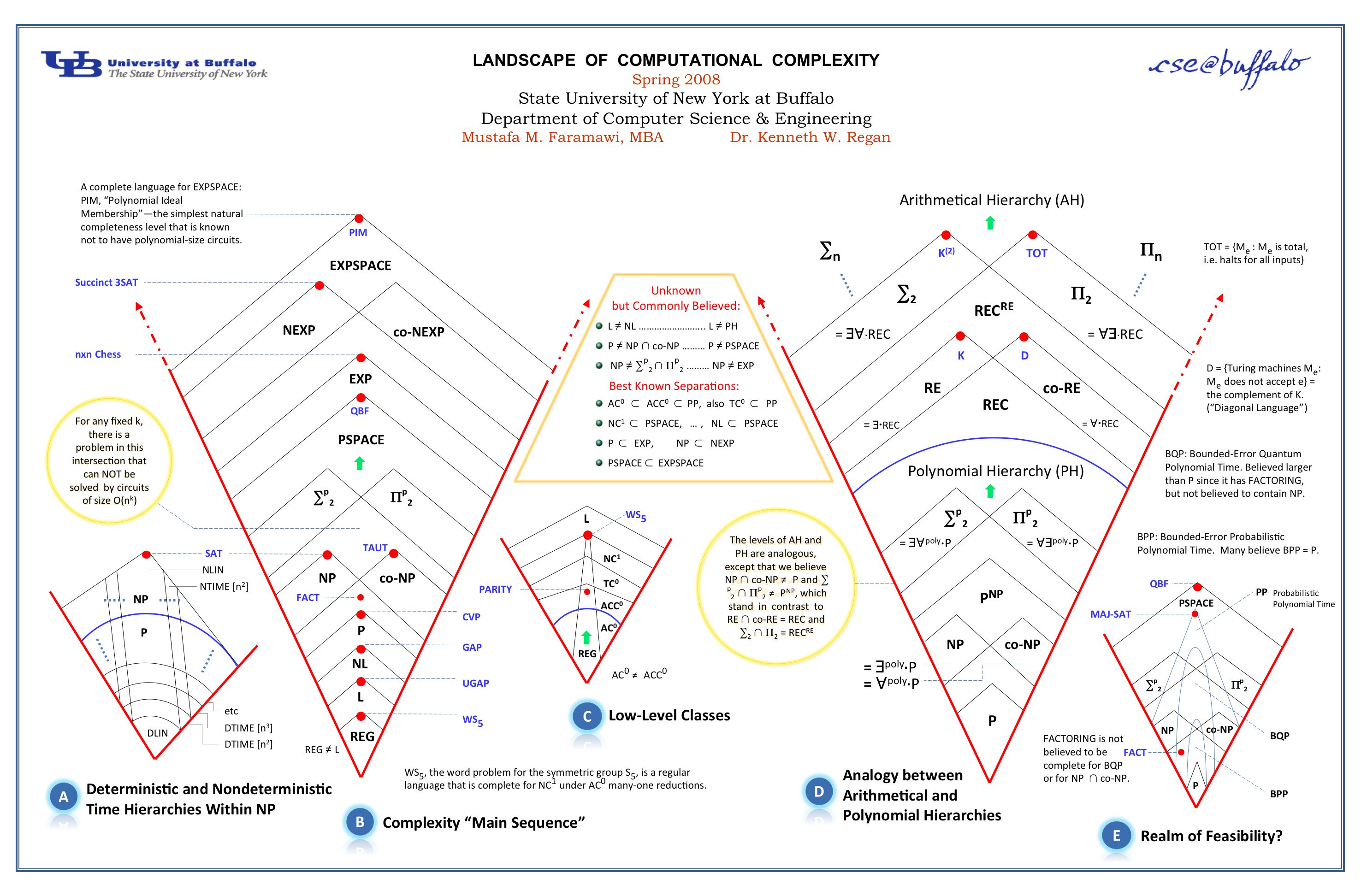
Interview circuit:
Error in interview circuit which is an NC sorting network with PSPACE-complete voter interviews as inputs is defined in usual sense as: False positives + False negatives + False questions = Percentage of wrong answers marked as right + Percentage of right answers marked as wrong + Percentage of wrong questions
For sorting purposes output of TQBF is not a binary 0 or 1 but a binary string with value equal to number of correct answers. Like all other boolean functions sensitivity of TQBF phi(q1,a1,q2,a2,q3,a3,…,qn,an) is defined as how flipping of qi and ai affects the output. Formally,
Sensitivity(TQBF) = Pr(TQBF(X) != TQBF(Xcorrelated)) where Xcorrelated is an interview with erroneous questions and answers.
Thus sensitivity captures the error in interview. It has to be noted that wrong questions also measure the flaw in interview process while wrong answer to a right question is already accounted for by a binary 0. When sensitivity of TQBF is 0, interview is flawless and LHS if P(good) is 1. BKS Majority is least stable conjecture by [Benjamini-Kalai-Schramm] predicts existence of a linear threshold function with stability greater than Majority function of n variables, n odd. Interview Circuit which is a composition of an NC sorting network with PSPACE TQBF interviews of voters, is also a linear threshold function which outputs candidate above a threshold (i.e sum of correct answers > threshold). If Stability(Interview) > Stability(Majority) then it is a proof of BKS conjecture. For large n, Stability(Majority) = 1-2/pi*(delta). When delta is close to 1, Stability(Majority) tends to 0.35.
Pseudorandom Choice:
Set of all voter decision functions is partitioned into n sets where each set has goodness xi. Here goodness of a voter decision function f is defined as: 1-error(f).
Let number of voter decision functions with goodness xi = m(xi). Thus N = m(x1)+m(x2)+m(x3)+…+m(xn) Expected goodness of a PRG choice is:
1/N * summation(xi*m(xi)) = (x1*m(x1) + x2*m(x2) + x3*m(x3) + … + xn*m(xn)) / N
When all voter functions have goodness 1 then PRG choice in LHS of P(good) has goodness 1.
These two non-majority choices are just hypothetical examples of how a social choice can be made without voting. In reality how non-majority social choice occurs is quite complex and determined by various factors of society ( economic disparities, ethnicity etc.,)
360. (FEATURE-DONE) Commits - 11 January 2017 - DeepLearning Convolution Networks update
Some changes done to Convolution computation: *) Made sigmoid perceptron optional in final neural network from Maxpooling layer so that weighted sum is printed instead of sigmoid value *) This causes the convolution network to be very sensitive to presence of pattern *) 2 more example bitmaps have been added with varying degree of pattern prominence (a pronounced X and a thin 1) *) With this final neurons from maxpooling layer print values of neurons which quite closely reflect the pattern’s magnitude: Huge pattern results in big value while small pattern results in small value proportionately. *) This can rank the bitmaps in increasing degree of magnitude of pattern presence *) Logs for this have been committed to testlogs
361. (FEATURE-DONE) DeepLearning Convolution Network - an example pattern recognition from bitmap images - 12 January 2017
*) Few more bitmap images have been included with same pattern but of different sizes *) There are 5 patterns and 9 bitmaps:
Thin X and Boldfaced X
Thin 0 and Boldfaced 0
Thin 8 and Boldfaced 8
No pattern
Thin 1 and Boldfaced 1
*) Expectation is that Convolution Network final neuron layer must output similar values for same pattern and different values for different patterns *) pooling_neuron_weight has been reintroduced in final neuron layer of 10 neurons each with a randomly chosen weight. *) Logs show for all 10 neurons, final neural activation values are close enough for similar patterns and different for different patterns. *) Thus Convolution Network which is a recent advance in DeepLearning works quite well to recognize similar image patterns.
In above example , 9th and 10th neurons output following values. Example 11 and 12 are similar patterns - 0 and 0. Example 21 and 22 are similar patterns - 8 and 8. Example 41 and 42 are similar patterns - X and X. Example 51 and 52 are similar patterns - 1 and 1. Neurons reflect this similarities :
Inference from Max Pooling Layer - Neuron 8
Example 11:
[27.402311485751664]
Example 12:
[27.36740767846171]
Example 21:
[32.15200939997122]
Example 22:
[30.835940458495205]
Example 3:
[17.133246549473675]
Example 41:
[29.367605168715038]
Example 42:
[27.446193773968886]
Example 51:
[22.12145242997834]
Example 52:
[24.17603022706531]
Inference from Max Pooling Layer - Neuron 9
Example 11:
[24.667080337176497]
Example 12:
[24.635666910615544]
Example 21:
[28.941808459974094]
Example 22:
[27.757346412645685]
Example 3:
[15.424921894526316]
Example 41:
[26.435844651843524]
Example 42:
[24.70657439657199]
Example 51:
[19.914307186980512]
Example 52:
[21.763427204358788]
362. (FEATURE-DONE) DeepLearning BackPropagation Implementation Update - 17 January 2017
*) DeepLearning BackPropagation code has been changed to have 3 inputs, 3 hidden and 3 output layers with 3*3=9 input-hidden weights and 3*3=9 hidden-output weights with total of 18 weights *) Software Analytics example has been updated with a third input and logs for it have been committed to testlogs/. *) Logs include a diff notes of how to extend this for arbitrary inputs and accuracy of backpropagation which beautifully converges at ~10^-26 error after ~1000000 iterations.
363. (FEATURE-DONE) Software Analytics with DeepLearning - 18 January 2017
*) An example software analytics code based on DeepLearning implementation has been added to software_analytics which import BackPropagation,Convolution and RecurrentLSTM to learn models from software analytics input variables (CPU%, Memory% and TimeDuration%) *) Logs for all 3 models learnt with same input variables have been added to software_analytics/testlogs
letter positions as y-axis and letter positions as x-axis. *) A sample polynomial plotted with matplotlib has been added to testlogs/ alongwith logs *) Once a text is plotted as a polynomial curve, it is natural to define distance between two strings as distance between two respective polynomial encodings. *) Usual distance measures for strings e.g Edit distance are somewhat qualitative and do not quantify in numeric terms exactly. *) Distance between polynomials of two texts is numerically quite sensitive to small changes in texts and visually match the definition of “distance” between two polynomials of strings.
There are two distance functions defined for polynomial representation of texts: *) Distance between polynomials is defined by inner product of polynomials f(x) and g(x) and in discrete version is the L2 norm : sum(i(f(xi)-g(xi))^2) *) Distance between polynomials considering them as two discrete set of probability distributions - Kullback-Leibler and Jensen-Shannon
Divergence measures.
text9=”fdjfjkkkkkkkkkkkkkfjjjjjjjjjjjskwwwwwwwwwwwwwwwwwwiiiiiiiiiiiiiiiiiiiiiiiiiiiiiiiiiiiiiiiiiiii” text10=”wjejwejwkjekwjkejkwjekjwkjekwjjoisjdiwidoiweiwie0iw0eio0wie0wie0iw0ei0cndknfndnfndnfkdjfkjdfkjd ——————————————————————————————————————————– X-axis: xrange(94) Y-axis: [102, 100, 106, 102, 106, 107, 107, 107, 107, 107, 107, 107, 107, 107, 107, 107, 107, 107, 102, 106, 106, 106, 106, 106, 106, 106, 106, 106, 106, 106, 115, 107, 119, 119, 119, 119, 119, 119, 119, 119, 119, 119, 119, 119, 119, 119, 119, 119, 119, 119, 105, 105, 105, 105, 105, 105, 105, 105, 105, 105, 105, 105, 105, 105, 105, 105, 105, 105, 105, 105, 105, 105, 105, 105, 105, 105, 105, 105, 105, 105, 105, 105, 105, 105, 105, 105, 105, 105, 105, 105, 105, 105, 105, 105] Coefficients of fitting polynomial of degree 5: [ 1.07744279e+02 -1.44951431e+00 1.33928005e-01 -3.69850703e-03
4.03119671e-05 -1.53297932e-07]
X-axis: xrange(95) Y-axis: [119, 106, 101, 106, 119, 101, 106, 119, 107, 106, 101, 107, 119, 106, 107, 101, 106, 107, 119, 106, 101, 107, 106, 119, 107, 106, 101, 107, 119, 106, 106, 111, 105, 115, 106, 100, 105, 119, 105, 100, 111, 105, 119, 101, 105, 119, 105, 101, 48, 105, 119, 48, 101, 105, 111, 48, 119, 105, 101, 48, 119, 105, 101, 48, 105, 119, 48, 101, 105, 48, 99, 110, 100, 107, 110, 102, 110, 100, 110, 102, 110, 100, 110, 102, 107, 100, 106, 102, 107, 106, 100, 102, 107, 106, 100] Coefficients of fitting polynomial of degree 5: [ 1.13816036e+02 -2.17630157e+00 1.96357195e-01 -6.45349037e-03
8.34267469e-05 -3.67775407e-07]
…
Two text polynomial ordinal points are represented as set of ordered pairs
Wagner-Fischer Edit Distance for text9 and text10: 76 Polynomial Encoding Edit Distance (JensenShannon) for text9 and text10: str1str2_tuple: [(102, 119), (100, 106), (106, 101), (102, 106), (106, 119), (107, 101), (107, 106), (107, 119), (107, 107), (107, 106), (107, 101), (107, 107), (107, 119), (107, 106), (107, 107), (107, 101), (107, 106), (107, 107), (102, 119), (106, 106), (106, 101), (106, 107), (106, 106), (106, 119), (106, 107), (106, 106), (106, 101), (106, 107), (106, 119), (106, 106), (115, 106), (107, 111), (119, 105), (119, 115), (119, 106), (119, 100), (119, 105), (119, 119), (119, 105), (119, 100), (119, 111), (119, 105), (119, 119), (119, 101), (119, 105), (119, 119), (119, 105), (119, 101), (119, 48), (119, 105), (105, 119), (105, 48), (105, 101), (105, 105), (105, 111), (105, 48), (105, 119), (105, 105), (105, 101), (105, 48), (105, 119), (105, 105), (105, 101), (105, 48), (105, 105), (105, 119), (105, 48), (105, 101), (105, 105), (105, 48), (105, 99), (105, 110), (105, 100), (105, 107), (105, 110), (105, 102), (105, 110), (105, 100), (105, 110), (105, 102), (105, 110), (105, 100), (105, 110), (105, 102), (105, 107), (105, 100), (105, 106), (105, 102), (105, 107), (105, 106), (105, 100), (105, 102), (105, 107), (105, 106), (1, 100)] 421.059610023 Polynomial Encoding Edit Distance (L2 Norm) for text9 and text10: str1str2_tuple: [(102, 119), (100, 106), (106, 101), (102, 106), (106, 119), (107, 101), (107, 106), (107, 119), (107, 107), (107, 106), (107, 101), (107, 107), (107, 119), (107, 106), (107, 107), (107, 101), (107, 106), (107, 107), (102, 119), (106, 106), (106, 101), (106, 107), (106, 106), (106, 119), (106, 107), (106, 106), (106, 101), (106, 107), (106, 119), (106, 106), (115, 106), (107, 111), (119, 105), (119, 115), (119, 106), (119, 100), (119, 105), (119, 119), (119, 105), (119, 100), (119, 111), (119, 105), (119, 119), (119, 101), (119, 105), (119, 119), (119, 105), (119, 101), (119, 48), (119, 105), (105, 119), (105, 48), (105, 101), (105, 105), (105, 111), (105, 48), (105, 119), (105, 105), (105, 101), (105, 48), (105, 119), (105, 105), (105, 101), (105, 48), (105, 105), (105, 119), (105, 48), (105, 101), (105, 105), (105, 48), (105, 99), (105, 110), (105, 100), (105, 107), (105, 110), (105, 102), (105, 110), (105, 100), (105, 110), (105, 102), (105, 110), (105, 100), (105, 110), (105, 102), (105, 107), (105, 100), (105, 106), (105, 102), (105, 107), (105, 106), (105, 100), (105, 102), (105, 107), (105, 106), (1, 100)] 200.743617582 ################################################################################## From above, usual edit distance between 2 strings is less than polynomial distances of JensenShannon and L2 norms. Ordinal values were not normalized by subtracting lowest possible ordinal value of unicode.
367. (FEATURE-DONE) Berlekamp-Welch Algorithm implementation - update for text message decoding - 27 January 2017
*) Using unicode values for ordinals with ord() and inverting with chr() causes overflow errors in SciPy/NumPy Linear Algebra Equation solver (solve()) because evaluating polynomials for large messages creates huge numbers *) Hence unicode has been replaced with a simple dictionaries - alphanumeric to numeric values and numeric to alphanumeric values. *) With above 2 dictionaries an example text message with error (garbled version of “thisissentence”) is list decoded with a window of possible values for each letter positions. *) Logs show an approximate decoding of original message from message with error. *) Garbled text with error was created from a previous execution of Berlekamp-Welch algorithm.
369. (FEATURE-DONE) An experimental special case k-CNF SAT Solver algorithm implementation - 31 January 2017
Algorithm:
*) Create a k-DNF from k-CNF input by negating literals in all clauses of k-CNF *) Binary encode the clauses of k-DNF into set of binary strings of length n where n is number of variables *) Compute the complement of the previous binary encoded set from set of 2^n binary strings *) These are satisfying assignments *) Presently requires all literals in each CNF clause *) Implemented for simulation of a Majority Voting with Voter SATs
g(x) is for 0s colored blue. For example, 1001011 is a 2-colored sequence with red (1) in bit positions 1,4,6,7 and blue (0) in bit positions 2,3,5. Complement functions for this bit position binary coloring are defined as:
f(1)=1 f(2)=4 f(3)=6 f(4)=7
- and
g(1)=2 g(2)=3 g(3)=5
- Natually, arithmetic progressions and monochromatic arithmetic progressions on these bit positions can be defined. Discrepancy is the
difference between number of colored integers in an arithmetic progression. Roth’s estimate which is the minimum(maximum(discrepancy))
for all possible colorings (i.e all possible binary strings) is >= N^(1/4+epsilon). For majority function 2-coloring, this estimate is the difference between number of 0s and 1s in the input to majority function with probability equal to natural density of min(max()) arithmetic progression. If majority function outputs 1, |f(x)| > |g(x)| and if 0, |g(x)| > |f(x)|. From this an approximate estimate of number of 1s and 0s in majority function input can be obtained (with probability equal to natural density):
- and vice versa if majority function outputs 0. For previous example, majority is 1 and :
|f(x)| = number of 1s = [7 + 7^0.25]/2 = 4.313288 ~ 4 |g(x)| = number of 0s = [7 - 7^0.25]/2 = 2.6867 ~ 3
Sensitivity of Majority function is number of bits to be flipped to change the outcome which is nothing but the discrepancy (|f(x)| - |g(x)|) wth probability equal to natural density and is lowerbounded by Roth’s estimate. Formally, Sensitivity(Majority) > N^(1/4+epsilon). An important special case is when input to majority is a binary string 2-colored by prime-composite complement functions in bit positions i.e prime bit positions are 1 and composite bit positions are 0 and majority function outputs 0 or 1 (Approximate number of primes less than N = pi(N) ~ N/logN from Prime Number Theorem).
371. (FEATURE-DONE) Reinforcement Learning - ThoughtNet based Recommender Systems Implementation Update - 2 February 2017
*) Recursive Gloss Overlap classifier disambiguation has been updated to invoke NLTK lesk algorithm function() with options to choose between PyWSD lesk implementation and best_matching_synset() primitive disambiguation native implementation *) New usecase shopping cart example with book reviews has been added *) Fixed a major bug in RecursiveGlossOverlap Classifier in definition graph construction : Edges for all lemma names of previous level synsets were added which bloated the graph and somewhat skewed core number of the graph. Changed it to create edge only for one lemma name. All other Recursive Gloss Overlap implementations in InterviewAlgorithm/ folder already have this fix. Regenerated the hypergraph for shoppingcart3 example Logs for this have been added to testlogs/
372. (FEATURE-DONE) Recursive Gloss Overlap classifier update - 3 February 2017
Uncommented NetworkX matplotlib graph plotting to get a graph for a sample document definition graph. Logs and PNG file for this classification have been added to testlogs/. Also did some experimentation with various documents and classification based on core number has been reasonably accurate (relevance of unsupervised core number based classification to the document’s actual class decreases with core number) and top percentage classes reflect the subject matter of the document. Also best_matching_synset() lesk disambiguation implemented in AsFer and NLTK lesk() functions are faster than PyWSD simple_lesk().
373. (THEORY and FEATURE-DONE) CNFSAT solver update - polynomial time approximation - 5 February 2017
- Solves CNFSAT by a Polynomial Time Approximation scheme:
Encode each clause as a linear equation in n variables: missing variables and negated variables are 0, others are 1
Solve previous system of equations by least squares algorithm to fit a line
Variable value above 0.5 is set to 1 and less than 0.5 is set to 0
Rounded of assignment array satisfies the CNFSAT with high probability
Essentially each CNF is represented as a matrix A and solved by AX=B where X is the column vector of variables and B is identity column vector
374. (FEATURE-DONE) Java Spark Streaming - Generic Stream Receiver Implementation - 6 February 2017
Spark Streaming Java implementation to receive generic stream of unstructured text data from any URL and Sockets has been added to NeuronRain AsFer java/bigdata_analytics/. It is based on Spart 2.1.0 + Hadoop 2.7 single node cluster. Following are the setup prerequisites:
) Oracle Java 8 compiler and runtime and PATH set to it *) export CLASSPATH=/home/shrinivaasanka/spark-2.1.0-bin-hadoop2.7/jars/spark-streaming_2.11-2.1.0.jar:.:/home/shrinivaasanka/spark-2.1.0-bin-hadoop2.7/jars/scala-library-2.11.8.jar:/home/shrinivaasanka/spark-2.1.0-bin-hadoop2.7/jars/spark-sql_2.11-2.1.0.jar:/home/shrinivaasanka/spark-2.1.0-bin-hadoop2.7/jars/spark-core_2.11-2.1.0.jar:/usr/lib/jvm/java-8-oracle/bin:/usr/local/sbin:/usr/local/bin:/usr/sbin:/usr/bin:/sbin:/bin *) Compiled as: javac SparkGenericStreaming.java *) JAR packaging of SparkGenericStreaming.class : jar -cvf sparkgenericstreaming.jar *class *) Example Spark submit commandline for 2 local threads (2 cores) and data streamed from twitter : /home/shrinivaasanka/spark-2.1.0-bin-hadoop2.7/bin/spark-submit –class SparkGenericStreaming –master local[2] sparkgenericstreaming.jar “https://twitter.com/search?f=tweets&vertical=news&q=Chennai&src=typd”
Spark Streaming Java implementation complements Streaming Abstract Generator Python native abstraction implemented in AsFer. Advantage of Spark Streaming is it can process realtime streamed data from many supported datasources viz.,Kinesis,Kafka etc., This implementation is generic, customized for arbitrary streaming data.
375. (FEATURE-DONE) Java Spark Streaming for Generic data - Jsoup ETL integration - 7 February 2017
*) Jsoup HTML parser has been imported into SparkGenericStreaming.java and a very basic Extract-Transform-Load is performed on the URL passed in with a special boolean flag to use Jsoup *) Jsoup connects to URL and does a RESTful GET of the HTML, extracts text from HTML and stores the text in Spark RDD *) receive() is periodically invoked and word count is computed *) foreachRDD() is invoked on the DStream to iterate through all words in DStream. *) forEach() invokes a lambda function to print the word text *) Logs for this have been added to spark_streaming/testlogs/
spark-submit commandline requires additional classpath to jsoup .jar with –jars option as below: /home/shrinivaasanka/spark-2.1.0-bin-hadoop2.7/bin/spark-submit –class SparkGenericStreaming –master local[2] –jars /home/shrinivaasanka/jsoup/jsoup-1.10.2.jar sparkgenericstreaming.jar “https://twitter.com/search?f=tweets&vertical=news&q=Chennai&src=typd” 2>&1 > testlogs/SparkGenericStreaming.out.7February2017
377. (FEATURE-DONE) Java Spark Streaming Generic Receiver update - 9 February 2017
*) Objectified the SparkGenericStreaming more by moving the SparkConf and JavaStreamingContext into class private static data. *) new method SparkGenericStreamingMain() instantiates the Spark Context and returns the JavaPairDStream<String,Integer> wordCounts object *) main() static method instantiates SparkGenericStreaming class and receives wordCounts JavaPairDStream from SparkGenericStreamingMain() method *) Spark JavaStreamingContext output operations are invoked by start() and print actions by lambda expressions. *) SparkConf and JavaStreamingContext variables have to be static because Not Serializable exceptions are thrown otherwise. *) sparkgenericstreaming.jar has been repackaged by recompilation.
*) DataFrame has been persisted to filesystem as .parquet file in overwrite mode of DataFrameWriter *) DataFrame has also been persisted to Hive MetaStore db which Spark supports (Shark SQL) with saveAsTable() *) SparkGenericStreaming has been rewritten to do transformations on words JavaRDD iterable with VoidFunction() in 2-level nested iterations of foreachRDD() and forEach() *) map() transformation for each row in JavaRDD throws a null pointer exception and inner call() is never invoked. *) This has been remedied by replacing map() with a forEach() and storing the rows in each RDD in an ArrayList *) With Hive MetaStore + Shark integration, Streaming_AbstractGenerator.py abstraction now has access to Java Spark Streaming because it already supports Hive via thrift and NeuronRain now has ability to analyze any realtime or batch unstructured data. *) Primitive ETL to just scrape words in URL text sufficiently tracks trending topics in social media. *) Hive metastore db, Spark warehouse data have been committed and Logs for this has been added to testlogs/ *) sparkgenericstreaming.jar has been repackaged with recompilation *) Updated spark-submit commandline: /home/shrinivaasanka/spark-2.1.0-bin-hadoop2.7/bin/spark-submit –class SparkGenericStreaming –master local[2] –jars /home/shrinivaasanka/spark-2.1.0-bin-hadoop2.7/jars/scala-reflect-2.11.8.jar,/home/shrinivaasanka/spark-2.1.0-bin-hadoop2.7/jars/spark-catalyst_2.11-2.1.0.jar,/home/shrinivaasanka/jsoup/jsoup-1.10.2.jar sparkgenericstreaming.jar “http://www.facebook.com” *) Updated CLASSPATH: export CLASSPATH=/home/shrinivaasanka/spark-2.1.0-bin-hadoop2.7/jars/scala-reflect-2.11.8.jar:/home/shrinivaasanka/spark-2.1.0-bin-hadoop2.7/jars/spark-catalyst_2.11-2.1.0.jar:/home/shrinivaasanka/jsoup/jsoup-1.10.2.jar:/home/shrinivaasanka/spark-2.1.0-bin-hadoop2.7/jars/spark-streaming_2.11-2.1.0.jar:.:/home/shrinivaasanka/spark-2.1.0-bin-hadoop2.7/jars/scala-library-2.11.8.jar:/home/shrinivaasanka/spark-2.1.0-bin-hadoop2.7/jars/spark-sql_2.11-2.1.0.jar:/home/shrinivaasanka/spark-2.1.0-bin-hadoop2.7/jars/spark-core_2.11-2.1.0.jar:/usr/lib/jvm/java-8-oracle/bin:/usr/local/sbin:/usr/local/bin:/usr/sbin:/usr/bin:/sbin:/bin
if (u,v) is in E(G1) then (f(u),f(v)) is in E(G2)
for recursive gloss overlap graphs G1 and G2 for languages L1 (e.g. English) and L2 (e.g Tamizh) constructed from respective ontologies. In previous definition, u and v are two words in natural language L1 and f(u) and f(v) are two words in natural language L2. This relaxes the isomorphism requirement mentioned in 178. Set of all digraphs G such that there is a homomorphism from G to a graph H is denoted by L(H). Guessing the set of digraphs G for a digraph H implies finding set of all translations for a text from a set of natural languages to another natural language. This guessing problem is known by Dichotomy Conjecture to be either in P or NP-Complete.
380. (FEATURE-DONE) Approximate SAT solver update - 14 February 2017
*) Changed number of variables and clauses to 14 and 14 with some additional debug statements. *) After 4000+ iterations ratio of random 3SAT instances satisfied is: ~70%
381. (FEATURE-DONE) Java Spark Streaming with NetCat WebServer update and some analysis on HiveServer2+Spark Integration - 18 February 2017
*) Rewrote SparkGenericStreaming.java mapreduce functions with Spark 2.1.0 + Java 8 lambda functions *) Enabled Netcat Socket streaming boolean flag instead of URL socket with Jsoup *) With above changes (and no HiveServer2), socket streaming receiver works and Hive saveAsTable()/Parquet file saving works. *) HiveServer2 was enabled in Spark Conf by adding hive-site.xml in spark/conf directory. (Two example hive-site.xml(s) have been committed to repository.) *) Spark 2.1.0 was started with hive-site.xml to connect to HiveServer2 2.1.1. This resulted in 2 out of heapspace errors as documented in testlogs/ with exception “Error in instantiating HiveSessionState”. *) Such OOM errors with HiveServer2 and Spark have been reported earlier in Apache JIRA. Instead of TTransport, FrameTransport was also tried which caused “Frame size exceeds maximum frame size” errors. SASL was also disabled in hive-site.xml. *) Reason for such OOM errors in HiveServer2 seems to be heavy memory footprint of HiveServer2 and Spark together and CPU usage reaches 100% for both cores. Might require a high-end server with large RAM size so that heapspace is set to atleast 8GB. HiveServer2 is known to be memory intensive application. Also Spark only supports Hive 1.2.1 and not Hive 2.1.1 which could be the reason. *) Increasing Java Heap space in spark config file (spark.executor.memory and spark.driver.memory) also did not have effect. *) Setting HADOOP_HEAPSIZE also did not have effect. OOM error occurs while instantiating HiveSessionState and bootstrapping Hive databases (get_all_databases). Isolated beeline CLI connection works though with HiveServer2. *) Hence presently Spark Streaming works with Spark provided metastore_db Hive Support and Parquet file support. *) testlogs/ have stream processing logs for NetCat (NC) webserver.
*) Earlier these were benchmarked with Spark 1.5.x *) Added debug statements in python-src/DiscreteHyperbolicFactorizationUpperbound_Bitonic_Spark.py and file locations updated. Logs committed to python-src/testlogs and python-src/InterviewAlgorithm/testlogs
384. (THEORY) Neural Tensor Networks Reasoning and Recursive Gloss Overlap merit scoring - 23 February 2017
Neural Tensor Networks described in 384.1 generalizes a linear neuron into a multidimensional tensor and assigns a score for relation between two entities e1 and e2. This is described in the context of an ontology (e.g WordNet) where a relation between two words w1 and w2 is assigned a score based on various distance measures. Recursive Gloss Overlap graph which is a gloss definition graph has a single relation between any two words - w1 “is in dictionary/gloss definition of” w2. Present implementation does not quantify the extent of relatedness between two words connected by an edge in Recursive Gloss Overlap graph. This definition graph can be considered as a Neural Tensor Network and each edge can be scored as a neural tensor relation between two word vertices. Cumulative sum total score of all edges in this graph is a quantitative intrinsic merit measure of the meaningfulness and intrinsic merit. Thus any document’s definition graph is a set of tensor neurons which together decide the merit of the text. Together with Korner Entropy complexity measure, Sum of Tensor Neuron scores effectively weight the text.
References:
384.1 Neural Tensor Networks - [SocherManningNg] - http://nlp.stanford.edu/pubs/SocherChenManningNg_NIPS2013.pdf
386. (FEATURE-DONE) Java Spark Generic Streaming and Streaming Abstract Generator Integration - 27 February 2017
*) Enabled URLSocket in Spark Generic Streaming and crawled an example facebook and twitter streaming data stored into Parquet files and Spark metastore *) Added Spark Streaming Data Source and Parquet Data Storage to Streaming_AbstractGenerator.py and updated iterator to read DataFrames from word.parquet Spark Streaming storage. *) Spark DataFrames are iterated by accessing word column ordinal and yielded to any application of interest. *) As an example Streaming HyperLogLogCounter implementation has been updated to read from Spark Parquet streaming data storage and cardinality is computed *) Example Spark Generic Streaming logs with URLSockets and HyperLogLogCounter with Spark Parquet data storage have been added to testlogs in python-src and java-src/bigdata_analytics/spark_streaming/testlogs *) Thus an end-to-end Java+Spark+Python streaming ETSL pipeline has been implemented where:
Extract is done by JSoup crawl
Transform is done by Spark RDD transformations
Store is done by Spark Hive and Parquet storage
Load is done by Streaming Abstract Generator iterator/facade pattern
*) Streaming_HyperLogLogCounter.py instantiates SparkSession from pyspark.sql. Usage of SparkSession requires executing this through spark-submit (Usual python <file> commandline doesnot work) as below: /home/shrinivaasanka/spark-2.1.0-bin-hadoop2.7/bin/spark-submit Streaming_HyperLogLogCounter.py 2>&1 > testlogs/Streaming_HyperLogLogCounter.out.SparkStreaming.27February2017
387. (FEATURE-DONE) Streaming Algorithms Implementations for Spark Streaming Parquet Data Storage - 28 February 2017
*) All Streaming_<algorithm> implementations have been updated to have Spark Streaming Parquet file storage as input generators. *) New Streaming_SocialNetworkAnalyis.py file has been added to do sentiment analysis for Streaming Data from Spark Parquet file storage *) Streaming_AbstractGenerator.py has been updated to filter each Spark Parquet DataFrame to remove grammatical connectives and extract only keywords from streamed content *) Logs for all Streaming_<algorithm>.py and Streaming_SocialNetworkAnalysis.py executed against Spark Streaming Parquet data have been committed to testlogs/ *) Streaming_SocialNetworkAnalysis.py presently iterates through word stream generated by Streaming_AbstractGenerator.py and does Markov Random Fields Clique potential sentiment analysis. *) Streaming_AbstractGenerator.py Spark Parquet __iter__() clause presently returns word stream which can be optionally made to return sentences or phrases of specific length *) All python streaming implementations instantiating Streaming_AbstractGenerator.py have to be executed with $SPARK_DIR/bin/spark-submit
388. (FEATURE-DONE) Major rewrite of BackPropagation Implementation for arbitrary number of Neuron input variables layer - 2 March 2017
*) BackPropagation algorithm code has been rewritten for arbitrary number of input layer, hidden layer and output layer variables. *) Some Partial Differential Equations functions have been merged into one function. *) This was executed with 6 variable input layer neuron, 6 variable hidden layer and 6 variable output layer with 2*6*6=72 weights for each of 72 activations. *) Logs for this have been committed to testlogs/ *) For 100000 iterations, error tapers to ~10^-29 as below ————————————————————————————————————– Error after Backpropagation- iteration : 99998 1.05827458078e-29 Layers in this iteration: ############### Input Layer: ############### [0.23, 0.11, 0.05, 0.046, 0.003, 0.1] ############### Hidden middle Layer: ############### [0.07918765738490302, 0.17639329000539292, 0.3059104560477687, 0.06819897810162112, 0.13596389556531566, 0.18092367420130773] ############### Output Layer: ############### [0.29999999999999977, 0.53, 0.11000000000000039, 0.09000000000000002, 0.010000000000004578, 0.2099999999999999] Weights updated in this iteration: [0.048788506679748, 0.11426171324845727, 0.24603459114714846, 0.0795780558315572, 0.17784209754093078, 0.18901665972998824, 0.11262698024008909, 0.20899193850252168, 0.5190303819914409, 0.3056462222980023, 0.5043023226568699, 0.6597581902164429, 0.16317511417689112, 0.6856596163043989, 1.0387023103855846, 0.2606362555325616, 0.9902995852922012, 1.0606233996394616, 0.03792106334721366, 0.08894920940249851, 0.19690317303590538, 0.06956852060077344, 0.15685074966243606, 0.1617685764906898, 0.07393365494416165, 0.11785754559950794, 0.32914500297950156, 0.2691055311488234, 0.4255090307780099, 0.5588219323805761, 0.17422407739745155, 0.7118075853635217, 0.335920938970278, 0.08421750448989332, 0.18955175416917805, 0.2131459459234997, 0.18585916895619456, 0.2871421205369935, 0.4097382856269691, 0.09927665626493291, 0.2820455537957722, 0.44170499922267087, 0.4181874495051114, 0.6343547541074734, 0.5019659876526656, 0.6341824150669009, 0.9311854573920668, 0.415739542966714, 0.8116648622103757, 0.7642211240783323, -0.27787045024304763, -0.03796350343576473, -0.06897746410924578, -0.12106324365840128, 0.09688102161356603, 0.0833653488478167, 0.025844281679456543, 0.01924251728820474, 0.1166534752079898, 0.22544113767193752, 0.2565459528164421, 0.2598246679566054, -0.2448286735461752, 0.48545168615654455, -0.12033616818940464, -0.17996884551601777, 0.09161370830913909, 0.16523481156548922, 0.22079944846849042, 0.4246703906819317, 0.05813513760785996, 0.49187786590191596] Recomputing Neural Network after backpropagation weight update Error after Backpropagation- iteration : 99999 1.05827458078e-29 Layers in this iteration: ############### Input Layer: ############### [0.23, 0.11, 0.05, 0.046, 0.003, 0.1] ############### Hidden middle Layer: ############### [0.07918765738490302, 0.17639329000539292, 0.3059104560477687, 0.06819897810162112, 0.13596389556531566, 0.18092367420130773] ############### ——————————————————————————————————————-
389. (FEATURE-DONE) Convolution Network Final Neuron Layer Integrated with BackPropagation Implementation- 3 March 2017
*) New python module has been added to repository to invoke BackPropagation algorithm implementation in final neuron layer of convolution network. *) This creates a multilayer perceptron from maxpooling layer variables as input layer and backpropagates for few iterations to do weight updates. *) Maxpooling layer is a matrix of 5*5=25 variables. With 25 variable input layer, backpropagation is done on 25*25*2=1250 activation edges with weights(25 inputs * 25 hidden + 25 hidden * 25 outputs). *) Logs for this have been added to testlogs/ *) Presently expected output layer has been hardcoded to some constant
reals too. Riemann Zeta Function and truth of Riemann Hypothesis imply a pattern in distribution of primes and hence pattern in prime-composite coloring. Thus Riemann Zeta Function is a 2-coloring scheme for set of natural numbers.
- Let q^s + q^(1-s) = v be an eigenvalue of a graph where s is a complex exponent (s=a+ib). It can be written as:
q^2s + q = vq^s q^2(a+ib) + q = vq^(a+ib) q^2a*q^2ib + q = vq^a*q^ib q^2a(e^i2blogq) + q = vq^a[e^iblogq] by rewriting q^ib = e^iblogq q^2a[cos(2blogq) + isin(2blogq)] + q = vq^a[cos(blogq) + isin(blogq)]
- Equating Re() and Im():
q^2a[cos(2blogq)] + q = vq^a[cos(blogq)] q^2a[sin(2blogq)] = vq^a[sin(blogq)]
- Ratio of Re() and Im() on both sides:
q^2a[sin(2blogq)] vq^a[sin(blogq)]
- ————————– = ——————
q^2a[cos(2blogq)] + q vq^a[cos(blogq)]
- q^2a[2*sin(blogq)*cos(blogq)] [sin(blogq)]
- ————————– = ——————
q^2a[cos(2blogq)] + q [cos(blogq)]
q^2a[2*cos(blogq)*cos(blogq)] = q^2a[cos(2blogq)] + q
q^2a[2*cos(blogq)*cos(blogq)] = q^2a[cos(blogq)*cos(blogq) - sin(blogq)*sin(blogq)] + q
q^2a[cos(blogq)*cos(blogq) + sin(blogq)*sin(blogq)] = q
q^2a = q => a = 0.5
When s=0.5 with no imaginary part and q+1 is regularity of a graph, v = 2*sqrt(q) and corresponding graph is a q+1 regular Ramanujan Graph.
[This is already derived in: https://sites.google.com/site/kuja27/RamanujanGraphsRiemannZetaFunctionAndIharaZetaFunction.pdf, https://sites.google.com/site/kuja27/RZFAndIZF_25October2014.pdf, http://sourceforge.net/p/asfer/code/HEAD/tree/python-src/ComplFunction_DHF_PVsNP_Misc_Notes.pdf]
Let H = {G1,G2,G3,…} be an infinite set of graphs with eigenvalues 1^s + 1^(1-s), 2^s + 2^(1-s), 3^s + 3^(1-s),….
Sum of these eigenvalues for infinite set of graphs has following relation to Riemann Zeta Function for s=w+1: Sum_q=1_to_inf(q^s + q^(1-s)) = [1 + 1/2^w + 1/3^w + …] + [1 + 2^(w+1) + 3^(w+1) + …] = RiemannZetaFunction + [1 + 2^(w+1) + 3^(w+1) + …]
Sum_q=1_to_inf(q^s + q^(1-s)) - [1 + 2^(w+1) + 3^(w+1) + …] = RiemannZetaFunction
Thus Riemann Zeta Function is written as difference of sum of eigenvalues for an infinite set of graphs and another infinite exponential series. Hermitian Real Symmetric matrices have real eigenvalues which is true for undirected graphs. For directed graphs, eigenvalues are complex numbers. Because of this condition, elements of set H have to be directed graphs. Relation between eigenvalues of two matrices M1 and M2 and eigenvalues of their sum M1+M2 is expressed by [Weyl] inequalities and [Knutson-Tao] proof of Horn’s conjecture. Sum of eigenvalues of M1+M2 is equal to sum of eigen values of M1 + sum of eigen values of M2 (Trace=sum of eigen values=sum of diagonal elements). The set H has one-to-one mapping with set of natural numbers and is 2-colored as prime and composite graphs based on index (each graph is monochromatic). Sum of adjacency matrices of H is also a directed graph (if all Gi have same number of vertices) denoted as G(H).
References:
390.1 Complex Analysis - [Lars Ahlfors] - Page 30 - Poles and Zeros, Page 213 - Product Development, Riemann Zeta Function and Prime Numbers 390.2 Honeycombs and Sums of Hermitian Matrices - http://www.ams.org/notices/200102/fea-knutson.pdf
391. (FEATURE-DONE) DeepLearning (ConvolutionNetwork-BackPropagation) JPEG files with Python Imaging Library (PILlow) - 6 March 2017
*) Added import of PIL Image library to open any image file and convert into a matrix in Integer mode *) This matrix is input to Convolution and BackPropagation code *) Logs of Convolution and BackPropagation for sample images have been committed to testlogs/
392. (FEATURE-DONE) DeepLearning (ConvolutionNetwork-BackPropagation) tobit() update - 7 March 2017
*) Updated python-src/DeepLearning_ConvolutionNetwork_BackPropagation.py tobit() function to map each pixel to a decimal value < 1 *) Increased BackPropagation iteration to 100. *) Logs for this have been committed to testlogs/. With this final neurons for max pooling layer are sensitive to changes in image pixels
393. (FEATURE-DONE) DeepLearning (ConvolutionNetwork-BackPropagation) image_to_bitmatrix() update - 8 March 2017
*) Refactored the tobit() function - moved it to a new directory image_pattern_mining and reimplemented it with a new image_to_bitmatrix() function in ImageToBitMatrix.py by enumerating through the pixel rows and applying map(tobit) *) This removed the opaqueness related 255 appearing for all pixels in bitmap. *) Each pixel is multiplied by a fraction. Mapping it to binary digits 0,1 based on [0-127],[128-255] intervals for pixel values does not work well with BackPropagation of MaxPooling in Convolution Network. Instead multiples of a small fraction makes the MaxPooling layer quite receptive to changes in image pixel values. *) Added few handwriting recognition example images for numbers 1(two fonts),2 and 8. *) Logs for this have been committed to testlogs/ ——————————————————— Following are Maxpooling Neurons ——————————————————— Final Layer of Inference from Max Pooling Layer - BackPropagation on Max Pooling Layer Neurons Inference from Max Pooling Layer - Image: [0.1452950826564989, 0.15731736449115244, 0.16984767785665972] Inference from Max Pooling Layer - Image: [0.14920888863234688, 0.16193600589418844, 0.17528092024601222] Inference from Max Pooling Layer - Image: [0.13197897244871004, 0.1417448800619895, 0.15171424525284838] Inference from Max Pooling Layer - Image: [0.14007345008310818, 0.15118749472569865, 0.16267822705412283] Inference from Max Pooling Layer - Image: [0.07847441088145349, 0.0807616625716103, 0.08303607840796547] Inference from Max Pooling Layer - Image: [0.08983732685398557, 0.09365789540391084, 0.09744765711798722] Inference from Max Pooling Layer - Image: [0.0903328782140764, 0.09421672093823663, 0.09806798136073994] Inference from Max Pooling Layer - Image: [0.08761036574911765, 0.09113121170496671, 0.09462405037074482] (‘Inference from Max Pooling Layer - Example 11:’, [0.1619896774094416, 0.1615169723530323, 0.15009965578039716]) (‘Inference from Max Pooling Layer - Example 12:’, [0.14303879829783814, 0.12068614560924568, 0.07211705852669059]) (‘Inference from Max Pooling Layer - Example 21:’, [0.1932801269861012, 0.11587916253160746, -0.007889615456070018]) (‘Inference from Max Pooling Layer - Example 22:’, [0.17605214289097237, 0.19326380725531284, 0.2114152778184319]) (‘Inference from Max Pooling Layer - Example 3:’, [0.062097695970929206, 0.062097695970929206, 0.062097695970929206]) (‘Inference from Max Pooling Layer - Example 41:’, [0.2976324086103368, 0.32891470561393965, 0.34986397693929844]) (‘Inference from Max Pooling Layer - Example 42:’, [0.22669904395788065, 0.26336097548290116, 0.3065443950445386]) (‘Inference from Max Pooling Layer - Example 51:’, [0.11935155170571034, 0.12477637373255022, 0.12911872514904305]) (‘Inference from Max Pooling Layer - Example 52:’, [0.12675869649313706, 0.12051203261825084, 0.10578392639393523]) ———————————————————- Previous logs are grep-ed from testlogs/. Handwritten Numeral recognitions (with high noise) are done in following Maxpooling inferences: [Number 1 - Font 1] Inference from Max Pooling Layer - Image: [0.07847441088145349, 0.0807616625716103, 0.08303607840796547] [Number 1 - Font 2] Inference from Max Pooling Layer - Image: [0.08983732685398557, 0.09365789540391084, 0.09744765711798722] [Number 2] Inference from Max Pooling Layer - Image: [0.0903328782140764, 0.09421672093823663, 0.09806798136073994] [Number 8] Inference from Max Pooling Layer - Image: [0.08761036574911765, 0.09113121170496671, 0.09462405037074482]
Contrasting this with bitmap numerals inscribed in 2 dimensional arrays (with low noise), similar elements have close enough values: [Number 0 - Font 1] (‘Inference from Max Pooling Layer - Example 11:’, [0.1619896774094416, 0.1615169723530323, 0.15009965578039716]) [Number 0 - Font 2] (‘Inference from Max Pooling Layer - Example 12:’, [0.14303879829783814, 0.12068614560924568, 0.07211705852669059]) [Number 8 - Font 1] (‘Inference from Max Pooling Layer - Example 21:’, [0.1932801269861012, 0.11587916253160746, -0.007889615456070018]) [Number 8 - Font 2] (‘Inference from Max Pooling Layer - Example 22:’, [0.17605214289097237, 0.19326380725531284, 0.2114152778184319]) [Null pattern] (‘Inference from Max Pooling Layer - Example 3:’, [0.062097695970929206, 0.062097695970929206, 0.062097695970929206]) [Letter X - Font 1] [(‘Inference from Max Pooling Layer - Example 41:’, [0.2976324086103368, 0.32891470561393965, 0.34986397693929844]) [Letter X - Font 2] (‘Inference from Max Pooling Layer - Example 42:’, [0.22669904395788065, 0.26336097548290116, 0.3065443950445386]) [Number 1 - Font 1] (‘Inference from Max Pooling Layer - Example 51:’, [0.11935155170571034, 0.12477637373255022, 0.12911872514904305]) [Number 1 - Font 2] (‘Inference from Max Pooling Layer - Example 52:’, [0.12675869649313706, 0.12051203261825084, 0.10578392639393523])
395. (FEATURE-DONE) Deep Learning Recurrent Neural Network Gated Recurrent Unit (RNN GRU) Implementation - 9 March 2017
*) This commit implements Gated Recurrent Unit algorithm (most recent advance in deep learning - published in 2014) which is a simplification of RNN LSTM by reducing number of gates (input, cell, forget, output are mapped to cell, reset, update) *) Logs for this have been uploaded to testlogs/ showing convergence of gates and state.
398. (FEATURE-DONE) Software Analytics update - 15 March 2017
*) Software Analytics Deep Learning code has been updated to include all Deep Learning implementations: RNN LSTM, RNN GRU, BackPropagation and ConvolutionNetwork+BackPropagation *) logs for this have been committed to software_analytics/testlogs/
399. (USECASE) NeuronRain Usecases - Software (Log) Analytics and VIRGO kernel_analytics config - 16 March 2017
Software Analytics Deep Learning implementation in python-src/software_analytics/ sources its input variables - CPU%, Memory%, TimeDuration% for a process from logs. VIRGO kernel_analytics module reads machine learnt config variables from kernel_analytics.conf and exports them kernelwide. An example single layer perceptron usecase is:
- If the CPU% is > 75% and Memory% > 75% and TimeDuration% > 75% then
do a kernelwide overload signal
- else
do nothing
- Sigmoid function for this usecase is:
sigma(4/9 * x1 + 4/9 * x2 + 4/9 * x3) where x1 = CPU%, x2 = Memory% and x3 = TimeDuration%
which is 1 when all variables reach 75%.
Spark Streaming Log Analyzer ETLs htop data to .parquet files and Software Analytics code reads it, deep-learns above neural network and writes a key-value variable OverloadSignal=1 to VIRGO kernel_analytics.conf. VIRGO kernel_analytics driver reads it and exports a kernelwide variable kernel_overload=1. Any interested kernel driver takes suitable action based on it (automatic shutdown, reboot, quiesce intensive applications etc.,)
An inverse of this usecase is to find the weights for x1,x2,x3 when system crashes. This requires a gradient descent or backpropagation with multilayered perceptron.
A simple example of strategic/tactical voting and Gibbard-Satterthwaite theorem is given in http://rangevoting.org/IncentToExagg.html. Here by changing the ranking preferences (i.e voter switch loyalties by manipulation, tactical and strategic voting, bribery, bounded rationality and erroneous decision etc.,) result of an election with atleast 3 candidates can be changed. Thus majority voting is vulnerable to error. Gibbard-Satterthwaite Theorem applies to all voting systems including secret ballot because even discreet voter can be psychologically influenced to change stance against inherent desire.
This implies for more than 3 candidates, RHS of P(Good) series for majority voting can never converge because there is always a non-zero error either by bounded rationality or manipulation. By pigeonhole principle either some or all of voters contributing to the P(Good) summation must have decided incorrectly or manipulated with non-zero probability. But this requires voter decision function (i.e social choice function) to be non-boolean (Candidates are indexed as 0,1,2,…). Exact learning of boolean functions applies to only 2 candidates setting where candidates are indexed as 0 and 1. Also, LHS of P(Good) series which is a (or quite close to a dictatorship by Friedgut-Kalai-Nisan quantitative version of Gibbard-Satterthwaite theorem) dictatorship social choice function, would be strategyproof (resilient to error and manipulative voting) and thus may have greater goodness probability (which is a conditional probability on chosen one’s goodness) than RHS in more than 3 candidates setting.
Condorcet Jury Theorem mentioned in references below, is exactly the P(Good) binomial series summation and has been studied in political science and social choice theory. This theorem implies majority decision is better and its goodness probability tends to 1 than individual decision if probability of correct decision making for each voter is > 0.5. In the opposite case majority decision goodness worsens if individual decision goodness probability is < 0.5. Thus majority voting is both good and bad depending on individual voter decision correctness. In terms of BP* complexity definitions, if each voter has a BP* social choice function (boolean or non-boolean) with p > 0.5, accuracy of majority voting tends to 100% correctness i.e Composition Majn(BPX1, BPX2,…) for some complexity class BPXi for each voter implying derandomization (this also implies BPX=X if Majn(BPX1,BPX2,…) composition is in BPX). Proof of BPP != P would imply there is atleast one voter with p < 0.5. Condorcet theorem ignores dependency and unequal error scenarios but still holds good by central limit theorem (because each voter decision is a random variable +1 or -1 and sum of these random variables for all voters tends to gaussian by CLT) and law of large numbers.
Corollary: From 129 and 368, depth of Majority voting circuit composition can be unbounded and if all voter social choice functions have same number of variables and number of voters is exponential in number of variables, Majority voting circuit composition with error is in BPEXP than PH. By Condorcet Jury Theorem, if all voters tending to infinity decide correctly with probability > 0.5, then BPEXP derandomizes to EXP => BPEXP=EXP. Non-boolean social choice functions for more than 2 candidates are usually preference profiles per voter (list of ranked candidates per voter) and topranked candidate is voted for by the voter.
If Majority Voting Circuit is in BPP, which is quite possible if number of voters is polynomial in number of variables and circuit is of polynomial size and because from Adleman’s Theorem (and Bennet-Gill Theorem), BPP is in P/poly, BPP derandomizes to P for infinite electorate with decision correctness probability > 0.5 for all voters. Thus homogeneous electorate of high decision correctness (> 0.5) implies both BPEXP=EXP and P=BPP.
- Locality Sensitive Hashing accumulates similar voters in a bucket chain. The social choice function is the distance function. Circuit/Algorithm for Multiway contest social choice (generalization of Majority boolean function) is:
*) Locality Sensitive Hashing (LSH) for clustering similar voters who vote for same candidate *) Sorting the LSH and find the maximum size cluster (bucket chain)
References:
400.1 Mechanism Design, Convicting Innocent, Arrow and GibbardSatterthwaite Theorems - https://ocw.mit.edu/courses/electrical-engineering-and-computer-science/6-254-game-theory-with-engineering-applications-spring-2010/lecture-notes/MIT6_254S10_lec21.pdf 400.2 Electoral Fraud, Gibbard-Satterthwaite Theorem and its recent extensions on manipulative and strategic voting, Cake cutting Multi Agent Resource Allocation Protocols - https://www.illc.uva.nl/COMSOC/theses/phd-schend.pdf 400.3 Condorcet Jury Theorem in Political Science - http://www.stat.berkeley.edu/~mossel/teach/SocialChoiceNetworks10/ScribeAug31.pdf - Asymptotic closed form and convergence of P(Good) binomial summation when probability of good decision > 0.5 uniformly for all voters was already solved by Condorcet 2 centuries ago :
“… Condorcet’s Jury theorem applies to the following hypothetical situation: suppose that there is some decision to be made between two alternatives + or −. Assume that one of the two decisions is ‘correct,’ but we do not know which. Further, suppose there are n individuals in a population, and the population as a whole needs to come to a decision. One reasonable method is a majority vote. So, each individual has a vote Xi , taking the value either +1 or −1 in accordance with his or her opinion, and then the group decision is either + or − depending on whether Sn = Pn i=1 Xi is positive or negative. Theorem 1.1. (Condorcet’s Theorem) [4] If the individual votes Xi , i = 1, … , n are independent of one another, and each voter makes the correct decision with probability p > 1 2 , then as n → ∞, the probability of the group coming to a correct decision by majority vote tends to 1. …”
400.4 Strategic Voting and Mechanism Design - [VinayakTripathi] - https://www.princeton.edu/~smorris/pdfs/PhD/Tripathi.pdf 400.5 Condorcet Jury Theorem and OCR - Section 2 - http://math.unipa.it/~grim/Jlamlouisa.PDF 400.6 Condorcet Jury Theorem graph plots - http://www.statisticalconsultants.co.nz/blog/condorcets-jury-theorem.html 400.7 Probabilistic Aspects of Voting - Course Notes - www.maths.bath.ac.uk/~ak257/talks/Uugnaa.pdf - Condorcet Jury Theorem, Bertrand Ballots Theorem and Gibbard Random Dictatorship Theorem 400.8 Law of Large Numbers and Weighted Majority - [Olle Haggstrom, Gil Kalai, Elchanan Mossel] - https://arxiv.org/abs/math/0406509v1 400.9 Thirteen Theorems in search of truth - http://www.socsci.uci.edu/~bgrofman/69%20Grofman-Owen-Feld-13%20theorems%20in%20search%20of%20truth.pdf - Condorcet Jury Theorem for Heterogeneous voters (voters with unequal decision correctness probability - Poisson-binomial distribution) - same as Condorcet Jury Theorem for Homogeneous voters (voters with equal decision correctness probability) when correctness probabilities are a Gaussian and > 0.5. In other words, large majority is more correct than small majority. 400.10 Margulis-Russo Formula and Condorcet Jury Theorem - http://www.cs.tau.ac.il/~amnon/Classes/2016-PRG/Analysis-Of-Boolean-Functions.pdf - pages 224-225 - Majority function is defined in Erdos-Renyi Random graph model with each edge having probability p. Maj(N,G) for a random graph G with probability of edge being p = True of G has atleast N/2 = |V|*(|V| - 1)/4 edges. Majority voting can be defined as a random graph with each voter being an edge with decision correctness probability p i.e Probability of Existence of an edge increases with correctness of decision by voter. Margulis-Russo formula describes the sharp threshold phenomenon for boolean functions and rate of change of P(Maj(G))=1 with respect to p, specifically for majority boolean function. Thus it is an alternative spectacle to view P(Good) majority voting binomial coefficient summation and Condorcet Jury Theorem. For majority function, sharp threshold occurs at p >= 0.5. 400.11 Percolation, Sharp Threshold in Majority, Condorcet Jury Theorem and later results, Influence, Pivotality - http://www.cs.tau.ac.il/~safra/PapersAndTalks/muligil.old.pdf 400.12 Complexity Inclusion Graph - https://www.math.ucdavis.edu/~greg/zoology/diagram.xml - BPEXP=EXP implies a significant collapse of the complexity class separation edges.
401. (FEATURE-DONE) LSH Index implementation for NeuronRain AsFer Text and Crawled Web Documents Intrinsic Merit Ranking - 4 April 2017
*) This commit adds a Locality Sensitive Hashing based inverted index for scrapy crawled HTML website pages. *) It is a derivative of LSH based similarity clustering implemented in python-src/LocalitySensitiveHashing.py *) It has to be mentioned here that ThoughtNet is also an inverted index for documents with additional features (i.e it is classifier based than raw string similarity) *) LSHIndex uses Redis Distributed Key Value Persistent Store as hashtable backend to store index. *) LSHIndex is not string to text inverted index, but hashed string to text inverted index (something like a digital fingerprint) *) Presently two types of hashes exist: primitive ordinal and MD5 hash *) Only one hash table is implemented on Redis with multiple hash functions with random choice. *) Presently 50 hash functions with 50 entries hash index has been implemented.
402. (FEATURE-DONE) ThoughNet Index implementation for NeuronRain AsFer Text and Crawled Web Documents Intrinsic Merit Ranking - 4 April 2017
*) This commit implements an inverted index on top of ThoughtNet *) ThoughtNet is a hypergraph stored in file and on Neo4j Graph Database *) JSON loads ThoughtNet edges and hypergraph files and queries by classes returned by Recursive Gloss Overlap classifier *) Querying Neo4j is also better, but file representation of ThoughtNet is quite succinct and scalable because it just numerically encodes each edge (= a web crawled HTML document) *) file representation of ThoughtNet views the hypergraph as stack vertices interconnected by document id(s) similar to a source code versioning system. Having similar view on a graph database doesn’t look straightforward
403. (FEATURE-DONE) Initial commits for Indexless Hyperball Recursive Web Crawler - 7 April 2017
*) An indexless crawler which tries to find a url matching a query string in a recursive crawl creating a hyperball of certain radius *) This is similar to Stanley Milgram, Kleinberg Lattice Small World Experiments and recent Hyperball algorithm for Facebook graph which concluded that Facebook has 3.74 degrees of freedom. *) Starts with a random url on world wide web. *) Success probability depends on average number of hops over large number of queries. *) This is a Randomized Monte Carlo Crawler and does a Depth First Search from an epicentre pivot url to start with *) Hyperball References:
405. (FEATURE-DONE) Commit - NeuronRain AsFer-CPython Extensions VIRGO64 system call invocations - 20 April 2017
*) VIRGO64 system calls are invoked from Python code by CPython extensions. *) Separate folder cpython_extensions64/ has been created for 64bit VIRGO kernel *) Requires Python 64-bit version *) Logs for VIRGO64 memory and filesystem systemcalls-to-drivers have been committed to testlogs *) With this Complete Application Layer-SystemCalls-Drivers request routing for python applications deployed on VIRGO64 works.
406. (FEATURE-DONE) Commits - NeuronRain AsFer Boost C++-Python - VIRGO64 System calls + Drivers invocation - 26 April 2017
*) VIRGO64 system calls are invoked from C++ by Boost::Python extensions *) Kernel Logs for VIRGO KMemCache, Clone and FileSystem Calls Boost::python invocations have been committed to testlogs/ *) Boost version used is 1.64.0 *) setup.py has been updated with library_dirs config variable *) virgofstest.txt for filesystem calls has been committed to testlogs/
407. (FEATURE-DONE) Commits - 28 April 2017 - NeuronRain AsFer-Boost::Python-C++ - VIRGO64 systemcalls and drivers invocations
*) VIRGO64 clone, kmemcache and filesystem system calls were invoked from Python-C++ boost extensions again and reproducibly work without kernel panics. *) Logs, persisted disk file written by filesystem system calls and rebuilt boost-python C++ extensions have been committed to testlogs/
More generically, vertex vx receives votes from vertices vy2,vy2,vy3,…,vyn with decision correctness probability p. Vertices vy1,vy2,vy3,…,vyn vote for vertices other than vx with decision correctness probability 1-p. Each vertex in WWW link graph has this 2 level tree structure with varying probability pi. From Condorcet Jury Theorem, hyperlinks to vx from vy1,vy2,…,vyn are 100% correct group decision if p > 0.5. Equal p for all votes to a vertex is the homogeneous voter assumption of Condorcet Jury Theorem. If the vertices are ranked by some algorithm (HITS Hub-Authority, PageRank etc.,) then correctness of rank is measured by Condorcet Jury Theorem. It is apt to mention here that probability p is different from weights of directed graph edges in PageRank Markov Random Walk iteration (where weight of outgoing edge/vote is decided by the ratio 1/outdegree) in the sense that: 1/outdegree is the static percentage of vote to an adjacent vertex in a non-random graph while p in network voting is a dynamic measure for decision correctness of a vote to a vertex in a random graph. For heterogeneous voter assumption, more recent theorems which generalize Condorcet Jury Theorem are required.
Collaborative Filtering in Recommender Systems is the most generalized way of Majority Voting where a matrix of users to their preferences for items is used as a training data for a new user to recommend an item. For example, if 9 out of 10 users up vote an item, 11th user is recommended that item and viceversa for down votes. Above analysis is an alternative direction for defining value judgement correctness already discussed in references 408.1 and 408.2. Correlated Votes and their effects on Condorcet Jury Theorem are analyzed by [KrishnaLadha].
References:
408.1 Condorcet Jury Theorem and the truth on the web - http://voxpublica.no/2017/03/condorcets-jury-theorem-and-the-truth-on-the-web 408.2 Webometrics, Goodness of PageRank and Condorcet Jury Theorem - [MastertonOlssonAngere] - https://link.springer.com/article/10.1007/s11192-016-1837-1 - PageRank is very good in finding truth i.e it is close to objective judgement with certain empirical assumptions despite being subjective ranking measure. Here objective judgement is any value judgement which is not majority voting or subjective. Computational linguistic text graph analysis which reckons the psychological aspects of text comprehension is an objective intrinsic merit judgement. Ideally majority vote should coincide with objective judgement absence of which implies error in voting or objective judgement or both (family of BP* complexity classes). 408.3 Generalized Condorcet Jury Theorem, Free Speech, Correlated Voting (dependence of voters) - https://www.jstor.org/stable/2111584
409. (FEATURE-DONE) Commits - 17 May 2017 - NeuronRain AsFer-VIRGO64 Boost-C++-Python invocations
*) Boost Python C++ VIRGO64 system calls were tested repeatedly in a loop *) All three system call subsystems - virgo_clone, virgo_kmemcache, virgo_filesystem - work well without any kernel panics *) But a strange thing was observed: virgo filesystem system calls were not appending to disk file but when run as “strace -f python asferpythonextensions.py” disk file is written to (a coincidence or strace doing something special)
411. (FEATURE-DONE) AngularJS - Tornado GUI-REST WebService - Commits - 1 June 2017
NeuronRain AngularJS RESTful client for Tornado webserver and others
*) AngularJS support has been added to NeuronRain GUI-WebServer with a new webserver_rest_ui/NeuronRain_AngularJS_REST_WebServer.py which reads and renders angularjs Model-View-Controller templates *) New AngularJS Model, View and Controller script-html templates have been added to angularjs directory *) LSHIndex.py has been updated to have commandline arguments for index queries *) Hyperball Crawler pivot epicentre url has been changed and an example query “Chennai” was found to be matching within few hops. *) NeuronRain_REST_WebServer.py has been updated to print the logs for the script execution to browser console with subprocess POpen() , communicate() and poll() python facilities
Rather than mere summation of potentials of edges following minmax criterion extracts the most meaningful random walk: *) Minimum Neuron Tensor Potential edge of each random walk is found - path minimum potential *) Maximum of all minimum path potentials extracts a random walk lambda composition tree which is the most probable inferred meaning of the document - Max(Min(potentials)) - this makes sense because maximum of minimum potential implies minimum possible neural activation.
Event Related Potentials (ERP) mentioned in 202 are unusual spikes in EEG of brain (N400 dataset) when unrelated words are read. Complement of ERP for related words as dataset could be an ideal estimator for Neuron Tensor relatedness potential between two words in definition graph.
Graph Neural Networks are recent models of neural network which generalize to a graph. In a Graph Neural Network, potential of each vertex is a function of potentials of all adjacent vertices and neuron tensor potentials of incoming edges from them. Neuron Tensor Network edge relations for each word vertices pair of Recursive Gloss Overlap Graph can be mapped to edges of a Graph Neural Network. Thus a text is mapped to not just a graph but to a Graph Neural Network with Tensor Neuron Edges, an ideal choice for human text comprehension simulation. Recursive Gloss Overlap Graph with Neuron Tensor word-word edges combines two concepts into one - Graph Tensor Neuron Network (GTNN).
Data on websites can be classified into 3 categories: 1) text 2) voice 3) images and videos. Intrinsic merit which is a measure of creativity presently focuses only on text. Analyzing the intrinsic merit of voice and visuals is a separate field in itself - Fourier Analysis of Waveforms and Discrete Fourier Transforms.
Ranking text by Graph Tensor Neuron Network intrinsic merit potential can be done in multiple ways: - Rank Vertices and Edges by potential - Rank the random walk lambda function composition tree by potential - Rank by Korner Entropy of the Graph Tensor Neuron Network and other qualitative and quantitative graph complexity metrics. and so on.
- Example lambda composition tree on a random walk of recursive gloss overlap graph:
f1 = requiredby(fuel, flight) f2 = has(flight, tyre) f3 = has(tyre, wheel) f4 = does(wheel, landing) f5 = requires(landing, gear) f1(fuel, f2(flight, f3(tyre, f4(wheel, f5(landing, gear)))))
Previous example random walk lambda composition tree has been constructed in 384 and 385. Potentials for Tensor Neuron Relations have to be predetermined by a dataset if such exists similar to N400 EEG dataset. Tensor Neuron Relations in Recursive Gloss Overlap Definition Graph are grammatical connectives mostly. In this example, “requiredby” is a relation. Cumulative potential of each such random walk lambda composition tree has to be computed.
Difference in Graph Tensor Neuron Network mapping of a text is: Each lambda composition tree is evaluated as a Graph Neural Network - each subtree is evaluated and passed on to higher level - and potential at the root is returned as the merit. Mixing time in markov chain andom walk is the number of steps before stationary distribution is attained. Thus maximum potential returned at the root of (a lambda composition graph tensor neuron network of (any converging stationary random walk of (a recursive gloss overlap definition graph of (a text)))) is a measure of intrinsic merit.
Intuition for Graph Tensor Neuron Network is below: *) Random walk on recursive gloss overlap graph simulates randomness in cognitive cerebral text comprehension. *) Tensor Neuron relatedness potential between two word vertices in definition graph quantifies relevance and meaningfulness *) Lambda composition tree-graph neural network for each random walk on definition graph simulates how meaning is recursively understood bottom-up with randomness involved.
References:
412.1 Graph Neural Networks - http://repository.hkbu.edu.hk/cgi/viewcontent.cgi?article=1000&context=vprd_ja
413. (FEATURE-DONE) Recursive Lambda Function Growth - Graph Tensor Neuron Network Implementation - Commits - 9 June 2017
(*) Recursive Lambda Function Growth implementation has been updated to compute Graph Tensor Neuron Network intrinsic merit (*) Each lambda function composition tree of a random walk on recursive gloss overlap graph is evaluated as a Graph Neural Network having Tensor Neuron potentials for word-word edges. (*) Tensor neuron potential for relation edges in Graph Neural Network has been hardcoded at present and requires a dataset for grammatical connective relations similar to EEG dataset for brain spikes in electric potentials.
414. (FEATURE-DONE) Graph Tensor Neuron Network - implementation update - Commits - 10 June 2017
*) Changed the subtree graph tensor neuron network computation
*) Children of each subtree are the Tensor Neuron inputs to the subtree root Each subtree is evaluated as a graph neural network with weights for each neural input to the subtree root.
*) WordNet similarity is computed between each child and subtree root and is presently assumed as Tensor Neuron relation potential for the lack of better metric to measure word-word EEG potential. If a dataset for tensor neuron potential is available, it has to to be looked-up and numeric potential has to be returned from here.
*) Finally a neuron activation function (simple 1-dimensional tensor) is computed and returned to the subtree root for next level.
*) logs for the this have been committed to testlogs. Presently graph tensor neuron network intrinsic merit is a very small decimal because of the decimal values of similarity and tensor neurons, but quite receptive to small changes.
*) Functions of classes have been parametrized for invocation across modules *) Both LSH and ThoughtNet indices have been recreated *) Ranking is done by Recursive Lambda Function Growth algorithm which is a superset of Recursive Gloss Overlap *) This script was tested via NeuronRain Tornado RESTful GUI
416. (FEATURE-DONE) Graph Tensor Neuron Network Intrinsic Merit and QueryIndexAndRank update - Commits - 15 June 2017
*) Graph Tensor Neuron Network Intrinsic Merit computation has been changed - Intrinsic merits of all random walks are summed up than multiplying to get a tangible merit value *) Some bugs fixed and debug prints have been changed *) logs have been committed to testlogs/
417. (FEATURE-DONE) Hyperball crawler update - Commits - 19 June 2017
Integrated Recursive Lambda Function Growth Intrinsic Merit Score(Graph Tensor Neuron Network and Korner Entropy) into Hyperball crawler.
418. (THEORY) Thought Experiment of Generic Intrinsic Merit and Condorcet Jury Theorem - 21 June 2017
Intrinsic merit so far is restricted to text documents. Subjective ranking measures are like mirrors which reflect the real merit of the candidate. Each vote in the majority voting is similar to an image of the votee projected on to the voter mirror. Some mirrors reflect well while others don’t. Efficiency of a voter mirror is equivalent to decision correctness of a voter. Present web ranking algorithms measure votee by the perception mirror images, which is indirect. Intrinsic merit breaks mirror images and relies only on what the votee really is. But then isn’t intrinisic merit a mirror image too? It is not because no human perception or image based voting is involved to ascertain merit. Only the graph complexity of the text-graph and its graph neural network is sufficient. Merit is a universal requirement. Examples in 410 and 202 motivate it. Can merit be applied to entities beyond voice, visuals and text? Most probably yes. Intelligence of human beings are ranked by intelligence quotients which is also an intrinsic merit measure (though IQ tests are disputed by psychological studies). Hence judging people by intrinsic merit is beyond just IQ scores. An algorithm to classify people as “Good” and “Bad” could be a breakthrough in machine intelligence. Hypothetical people classifier could be as below: (*) Peruse academic records and translate to score (*) Peruse work records and translate to score (*) Translate awards received to score (*) Translate brain imageing data to score (EEG and fMRI) (*) Translate IQ or EQ to score Above is not a formal algorithm but tries to intuit how it may look like. Human Resource Analytics are done as above
Objective Intrinsic Merit = Vote by an algorithm Subjective Ranking = Votes by people translated into rank by an algorithm (present ranking algorithms rely on incoming links or votes to a text which are created by human beings)
Thus Generic Intrinsic Merit removes human element completely while assessing merit (closer to AI).Goodness when it applies to human beings is not just a record based score and usually has moral and ethical elements in it. People classifier based on intrinsic merit has to be intrusive and invasive similar to HR analytics example earlier.
(*)Question: Why should intrinsic merit be judged only in this way? (*)Answer: This is not the only possible objective intrinsic merit judgement. There could be other ways too. Disclaimer is intrinsic merit assumes cerebral representation of sensory reception (words, texts, visuals, voices etc.,) and its complexity to be the closest to ideal judgement.
(*)Question: Wouldn’t cerebral representation vary from person to person and thus be subjective? (*)Answer: Yes, but there are standardized event related potential datasets gathered from multiple neuroscience experiments on human subjects. Such ERP data are similar for most brains. Variation in potential occurs because cerebral cortex and its sulci&gyri vary from person to person. It has been found that cortex and complexity of gray matter determine intelligence and grasping ability. Intrinsic merit should therefore be based on best brain potential data.
(*)Question: Isn’t perception based ranking enough? Why is such an intrusive objective merit required? (*)Answer: Yes and No. Perception majority voting based ranking is accurate only if all voters have decision correctness probability > 0.5 from Condorcet Jury Theorem. PageRank works well in most cases because incoming edges vote mostly with >50% correctness. This correctness is accumulated by a Markov Chain Random Walk recursively - vote from a good vertex to another vertex implies voted vertex is good (Bonacich Power Centrality) and so on. Initial goodness is based on weight of an edge. Markov iteration stabilizes the goodness. Probability that goodness of stationary Markov distribution < 0.5 can be obtained by a tail bound and should be exponentially meagre.
It was mentioned earlier that Fourier analysis of visuals and voice is the measure of intrinsic merit. Following definition of generic intrinsic merit further strengthens it: Generic intrinsic merit of an entity - text, visual or voice - is the complexity of cerebral representation potential as received by sensory perception. For texts it is the graph complexity measure. For voice and visuals it could ERPs activated on seeing or hearing and based on EEG data.
References:
418.1 Event Related Potentials for attractive facial recognition - https://labs.la.utexas.edu/langloislab/research/event-related-potential-erp/418.2 Event Related Potentials - http://cognitrn.psych.indiana.edu/busey/eegseminar/pdfs/Event-Related%2520PotentialsIntro.pdf - ERPs are cortical potentials of interoperating neurons in response to a cognitive stimulus.
421. (FEATURE-DONE) Text Summarization from Recursive Gloss Overlap Graph Core - Commits - 28 June 2017
(*) Added a new function to create a summary from text - This function creates the core of a Recursive Gloss Overlap graph with certain core number and writes out a text sentence for each edge in core subgraph obtaining least common ancestor(hypernym) relation (*) logs for this have been committed to python-src/testlogs
Summarization from k-core(s) of a Recursive Gloss Overlap graph captures the most crucial areas of the text because document belongs to the class/word vertex with high core numbers.
422. (FEATURE-DONE) Text Summarization from Recursive Gloss Overlap Graph Core - Commits - 30 June 2017
(*) New clause added to classify the text and match the prominent core number word vertices in the text and only add those sentences to summary. (*) This is an alternative to k-core subgraph traversal and creating text programmatically. It is based on the heuristic that a summary should capture the essence/classes the text belongs to. (*) Prominent core number classes are shaved off from the sorted core number list returned by RGO classifier and top percentile is used. Summary is limited in size relative to the original text.
423. (THEORY) Dense Subgraph Problem and Mining patterns in Graph Representation of Text - 2 July 2017
Recursive Gloss Overlap and Recursive Lambda Function Growth algorithms create graphs from text documents. Unsupervised classification from prominent vertices of the definition graph and Text summarization at present depend on finding k-core subgraphs. In general this is an NP hard problem to find Dense Subgraphs of a Graph where density of a subgraph S of a graph G is defined as:
d(S) = |Edges of S| / |Vertices of S|
There are polynomial time maxflow based algorithms and approximations to find dense subgraphs of a graph.
References:
423.1 Goldberg Algorithm, Charikar Algorithm and k-Cliques Densest Subgraph Algorithm for Dense Subgraph Discovery - people.seas.harvard.edu/~babis/dsd.pdf 423.2 Network Structure and Minimum Degree - [Social Networks - Seidman] - https://ucilnica.fri.uni-lj.si/pluginfile.php/1212/course/section/1202/Seidman%20-%20Network%20structure%20and%20minimum%20degree%2C%201983.pdf - k-cores as measure of connectedness in a network G which are maximal connected subgraphs of G whose vertices have degree atleast k.
426. (FEATURE-DONE) Updates to Text Summarization - Commits - 5 July 2017
(*) Changed the class-sentence matching clause by increasing the percentile of prominent classes (*) Changed relevance_to_text() by comparing each sentence chosen by prominent class match to the sentences in text - Ratcliff-Obershelp Longest Common Subsequence matching difflib library function is invoked for this similarity. Sentences are chosen also based on relevance_to_text() scoring (*) Percentage of summary to the size of the text has been printed as a ratio. Logs have been committed to testlogs/
427. (FEATURE-DONE) Updates to Text Summarization - choosing sentences matching class labels - 6 July 2017
(*) Some experimentation on choosing relevant sentences to be added to summary was performed (*) relevance_to_text() invocation has been changed as per algorithm below: for each prominent dense subgraph k-core class label find the synset definition of class label for each sentence invoke relevance_to_text() similarity function between sentence and the class label definition and add to summary if the relevance ratio > 0.41 and if not already in summary (*) Ratio 0.41 was arrived at heuristically: - For relevance ratio 0.1, summary ratio was 0.65 - For relevance ratio 0.2, summary ratio was 0.48 - For relevance ratio 0.3, summary ratio was 0.35 - For relevance ratio 0.4, summary ratio was 0.21 - For relevance ratio 0.5, summary ratio was 0.02 There is a drastic dip in size of summary if relevance threshold is increased beyond 0.4. Because of this 0.41 has been hardcoded. (*) Logs for this have been added to testlogs/ (*) Summary generated is human readable - subset chosen from actual text.
428. (FEATURE-DONE) ConceptNet 5.4 Python RESTful API implementation - lookup, search and association - 7 July 2017
(*) This commit implements the RESTful Python requests HTTP API for querying ConceptNet 5.4 dataset (*) Three functions for looking up a concept, searching a concept and finding similar associated concepts have been implemented with 3 endpoints (as per the documentation in https://github.com/commonsense/conceptnet5/wiki/API/2349f2bbd1d7fb726b3bbdc14cbeb18f0a40ef18) (*) ConceptNet is quite different from WordNet in representation as JSON dictionary as against graph in WordNet. (*) ConceptNet 5.4 endpoints have been invoked instead of 5. (*) If necessary ConceptNet can replace all WordNet invocations in a later point in time. But such a replacement is non-trivial and would probably require almost all Recursive Gloss Overlap related code to be rewritten from scratch. But that depends on how ConceptNet 5 weighs against WordNet in measuring semantic meaningfulness.
429. (THEORY) Contradictions in bounds between finite and infinite electorate - 8,10,11,12,13 July 2017
- Lowerbounds by equating the goodness of Non-majority and Majority social choice thus far mentioned in drafts in this document (subject to errors) are based on following assumptions:
(*) There are two possible paths to social choice - Non-majority and Majority (*) Each social choice belongs to a computational complexity class (*) Goodness of a social choice is the measure of error-free-ness of the choice made in either paths i.e decision correctness (e.g noise stability, sensitivity,error in BP* algorithm etc.,) (*) RHS Majority voting has been assumed to abide by Homegeneous version of Condorcet Jury Theorem convergence and divergence of group decision goodness as a function of individual voter goodness while LHS is either a pseudorandom choice or an interview TQBF algorithm (*) Goodness of either choice majority or non-majority must be equal (*) Either LHS or RHS has to be a complete problem for a complexity class C. (*) Traditional literature on boolean majority functions and circuits assumes that input to majority is readily available which is equivalent to SAT oracle access to Majority function where SAT oracle could belong to any complexity class (2-SAT, 3-SAT, k-QBFSAT, etc.,) => Majority voting is in P^NP,P^PH,P^EXP etc., (*) Previous Oracle access based proofs have been intentionally circumvented by replacing Oracles with Boolean Function/Circuit compositions which have strong Communication Complexity basis (KW relations and depth of a circuit composition mentioned in 368) (*) Assuming all above, LHS is an algorithm for RHS complete problem (or viceversa) creating a lowerbound. (*) All bounds derived in this draft assuming above do not follow conventional lowerbound techniques e.g Circuit Lower Bounds. Equal goodness assumption implies - “both algorithms solve same problem - one is more efficient than the other”. (*) Most importantly drafts in this document are just analyses of various social choice functions, their complexities and contradictions irrespective of attaining lowerbounds.
Equality of Goodness of PRG choice and Majority voting for finite electorate of size 3:
Let x1,x2,x3 be the goodness of 3 voter SATs. PRG choice randomly chooses one of the 3 voters while majority voting is the usual CJT Majority+SAT composition.
Goodness of PRG choice:
= (x1*m(x1) + x2*m(x2) + x3*m(x3)) / 3 When all 3 have equal goodness 1, effective goodness is: = (1*1 + 1*1 + 1*1)/3 = 1
Goodness of Majority choice:
This is the bounded version of CJT binomial series summation. When x1=x2=x3=1: = (3C2(1)^2(0)^1 + 3C3(1)^3(0)^0) = (0 + 1) = 1
Possible Lowerbounds described previously for Unbounded and Bounded electorate lead to contradictions as below: (*) In infinite voter case, homogeneous voter CJT circuit in BPP is derandomized to P if CJT converges => P=BPP. (*) In finite voter case, NP-complete RHS has BPP algorithm in LHS (NP in BPP) implying NP in P/poly and collapse of PH => NP in P/poly and PH in P/poly.
Contradiction 1 :
- If BPP=P (unbounded CJT) and NP is in BPP (bounded) then NP is in P=BPP => P=NP. This conflicts with P != NP implied by :
(*) the Majority Hardness Lemma (318), (*) Polytime learning of NP implying NP does not have polytime algorithms (368) and (*) HLMN PARITYSAT counterexample (53.15)
- but concurs with :
(*) high percentage of random k-SATs satisified in Approximate CNF SAT solver by least squares (376).
But can infinite voter CJT circuit be in BPP and thus in P/poly? Infinite voter CJT circuit is of polynomial size if it is polynomial in number of Voter SAT variables and exponential if it is exponential in number of variables. Latter happens only if all voters have dissimilar SAT variables while common variables across voter SATs make it exponential. This is described in example of 53.8. Condorcet Jury Theorem convergence in homogeneous voters case implies all voters are similar (e.g have similar voting SATs) thus ruling out polynomial size case i.e Unbounded CJT circuit can not both be in BPP and converging. This contradiction stems from the assumption - BPP derandomizes to P. LHS could be in RP too. RP is contained in NP. (Can BPP derandomize to NP i.e BPP in NP?). Another assumption is all voters have 3-SAT choice functions. If all voter SATs are 2-SATs (in P), infinite and finite voter cases are not equatable and there is no contradiction. Known result: If NP is in BPP, NP=RP - this applies to bounded voting case above. Thus BPP=P possibility is removed by exponential sized CJT circuit and BPEXP=EXP is still possible when CJT converges. Contradiction 1 is avoided.
Contradiction 2 :
If NP is in BPP and thus in P/poly (irrespective of BPP=P), similar conflicts arise. An assumption made in composition of 3-SAT voters and Majority function for bounded electorate in 424 is resultant composition is also in NP (depth lowerbound for this composition can be obtained by KW relations in 368). This assumption could be false because composition of NP 3-SAT with non-uniform NC1 majority function could be harder than mere NP - because this is equivalent to replacing oracle with a circuit composition in a P^NP algorithm. P with NP oracle adds an additional quantifier and places it in second level of polynomial hierarchy (inclusion in https://www.cse.buffalo.edu/~regan/papers/ComplexityPoster.jpg shows there are problems in Sigma(p,2) /Pi(p,2) which also have BPP algorithms and P^NP is contained in Sigma(p,2) /Pi(p,2)). Thus a PRG choice and converging bounded electorate voting of equal goodness need not imply NP in BPP. This composition may not be a complete problem. Stricter oracle definition of Majority+SAT composition is NC1(L) where Majority is computable by non-uniform circuits or BWBP with oracle access to gates belonging to a class L. For 3-SAT voter oracles, CJT majority voting circuit is in NC1(NP) (is this contained in P^NP?). Subject to equal goodness, composition equivalent of NC1(NP) is in BPP and not NP is in BPP.
Reference 429.3 suggests there exists a random oracle A relative to which NC^A is in P^A. P having NP oracle access is known as class delta(p,2)=P^NP. This answers if NC1^NP is in P^NP in the affirmative. There is a known delta(p,2)-complete problem mentioned in reference 429.5. If bounded electorate NC1^NP problem is complete for its class, then equal goodness of PRG choice and bounded majority voting implies NC1^NP is in BPP. This in turn implies NP is in BPP (if NC1^NP strictly contains NP) and thus NP is in P/poly again leading to contradiction in the outset.
- Replacing oracles with compositions and applying depth lowerbounds for Majority+VoterSAT circuit composition as below for m voters with n variables per voter SAT (from 368):
D(Maj + Voter) = CommunicationComplexity(R(Maj,Voter)) >= 5.3*logm + n - O(m*logm/n)
does away with the hassles of relativization and directly gives the depth lowerbound of the majority voting circuit composition. Size of this composition is the alternately phrased KRW conjecture in 429.7.
Example delta(p,2)-complete problem mentioned in 429.5:
While number of queries to NP oracle <= k {
(*) Query a 3SAT oracle for a satisfying assignment for a 3CNF Voter SAT (*) Store the queried satisfying assignment in a linked list in sorted order - this is linear per insertion i.e traverse the list and compare the two adjacent nodes. E.g. {1,5}, {1,3,5}, {1,3,5,6}, {1,3,5,6,7}… upto k-th query and lexicographic ordering is preserved by a decimal encoding of SAT oracle query string.
} Output 1 if last element in the list ends with binary 1 digit.
This algorithm makes k queries to an NP oracle and has O(k^2) time complexity and thus in delta(p,2). Hardness follows by reducing any polynomial time algorithm with NP oracle to above - reasonably straightforward because oracle queries are memoized and can be looked-up in polynomial time.
Mapping above delta(p,2) complete problem to proving completeness of NC1^NP majority voting is non-trivial. Majority function can make n queries to n voter SAT oracles and atleast n/2 + 1 queries should return 1 or 0 to compute majority in NC1. Beyond this, NC reducibility has to be proved by Many-one/Turing reductions or Logspace reductions of any other problem in NC1^NP to this. Integer multiplication,powering and division have been proved to be equivalent (NC reducible to each other) mentioned in reference 429.8. NC reducibility through oracle NC gates have been proved in reference 429.9. Majority function is known not to be complete for NC1 under AC0 many-instances-to-one reductions (reference 429.10). This could probably imply that NC1^NP is not complete too, thereby avoiding contradiction 2.
But this also implies that any Majority^A for a random oracle A is not complete if Majority is not complete for NC1. Hence it has to be proved or disproved if a problem is not NC1 complete, it is not NC1^A complete for an oracle A. Lemma 3.3.9 in reference 429.9 [RuzzoGreenlawHoover] describes an Oracle PRAM or an NC oracle circuit M’ to another NC circuit M. M has O(n^c) size/processors and depth/time of O(logn) and M makes at most O(n^c) oracle queries to M’ (each node can query). But these oracle queries are made simultaneously in parallel time of O(logn). Thus replacing calls to M’ by M’ itself increases depth by O(logn) and size by O(n^c) order of magnitude i.e new circuit without oracle M’ has time O((logn)^2) and size O(n^2c). Similar oracle replacement could be done for Majority^A circuits too. If oracle gates to Majority are replaced by circuit for A itself which has size s and depth d and Majority makes at most O(n^c) calls to oracle A, new Majority circuit without oracle has depth/time O(d*logn) and size/processors O(s*n^c). This new circuit need not be in NC1. From Spira’s Theorem a circuit of size O(s*n^c) can be transformed into a circuit of depth O(log(s*n^c))=O(log(s) + c*log(n)). Following cases arise after replacing oracle gates with a new circuit of size s.
Case 1 - s = 2^n:
This makes the new majority circuit sans oracle to be of depth O(n*log2+c*log(n)) which is not polylog depth and polynomial size and thus lies outside NC - this new circuit problem could be complete for a different class. This line of reasoning coincides with previous formulations of majority voting based on depth bounds by Communication Complexity (KRW Conjecture) and Direct Connect circuit families of unbounded depth and exponential size. If there is a problem B in NC1, Majority^A and B^A can be in totally different depth hierarchy classes by depth hierarchy theorem. This could be a complete problem in different class (e.g, PH-complete, EXP-complete etc.,) and can be equated under equal goodness assumption with a non-majority social choice.
Case 2 - s = n^c:
This new majority circuit has depth O(2*c*log(n)) and size O(n^2c) and is obviously in NC1 and computes majority. But majority is not complete for NC1 and thus majority voting itself is not a complete problem and cannot be equated under equal goodness assumption with a non-majority choice.
References:
429.1 Definition of Homogenenous Voter - http://www.uni-saarland.de/fak1/fr12/csle/publications/2006-03_condorcet.pdf - “…Now assume that a chamber consists of three homogenous judges. Homogenous means that the decision-making quality of each single judges is described by identical parameters r…” - identical parameters are translatable to identical variables though SAT could be different for each 429.2 Counting Classes and Fine Structure between NC and L - [Samir Datta , Meena Mahajan , B V Raghavendra Rao , Michael Thomas , Heribert Vollmer] - http://www.imsc.res.in/~meena/papers/fine-struct-nc.pdf - Definition of NC circuits with Oracle gates. Definitions 8 and 10 and Remark 9 - Majority NC1 circuit with NP oracle for all homogeneous voters belongs to Boolean Hierarchy and specifically is in NC1 hierarchy. 429.3 For a random oracle A, NC^A is strictly contained in P^A - https://complexityzoo.uwaterloo.ca/Complexity_Zoo:N, https://complexityzoo.uwaterloo.ca/Zooref#mil92 - [PeterBroMiltersen] 429.4 Delta(p,2) - P has NP oracle - https://complexityzoo.uwaterloo.ca/Complexity_Zoo:D#delta2p 429.5 Delta(p,2) complete problem - https://complexityzoo.uwaterloo.ca/Zooref#kre88 - [Krentel] - Given a Boolean formula, does the lexicographically last satisfying assignment end with 1? 429.6 Spira theorem - any formula of leaf size s can be transformed into a formula of depth log(s) - https://www.math.ucsd.edu/~sbuss/CourseWeb/Math267_1992WS/wholecourse.pdf 429.7 Size of a circuit composition - alternative form of KRW conjecture - http://www.math.ias.edu/~avi/PUBLICATIONS/GavinskyMeWeWi2016.pdf - “…This suggests that information complexity may be the “right” tool to study the KRW conjecture. In particular, since in the setting of KW relations, the information cost is analogous to the formula size, the “correct” way to state the KRW conjecture may be using formula size: L(g*f) ≈ L(g)·L(f)…” - for Majority+VoterSAT composition size is conjectured as O(n^5.3 * s) where s is the size of VoterSAT formula. Information complexity of a composition of a function g:{0,1}^m->{0,1} and a universal relation Un:{0,1}^n->{0,1} for majority voting is: a Voter SAT g of m variables is composed with a Majority universal relation of n variables. Majority is a universal relation because for 2 input strings to majority function drawn at random can be checked if they differ in a bit position. Above depth bound is the amount of mutual information “leaked” while computing the composition together by Alice and Bob. Alice gets a m*n matrix X and a string a in ginverse(0) and Bob gets a m*n matrix Y and a string b in ginverse(1) and both accept if a and b differ in a bit position and X and Y have row mismatch and reject else. ginverse(0) is equivalent to a rejecting assignment to SAT and ginverse(1) is equivalent to an accepting assignment to SAT because g() is the Voter SAT. 429.8 Log Depth circuits for Division and Related - [BeameCookHoover] - https://pdfs.semanticscholar.org/29c6/f0ade6de6c926538be6420b61ee9ad71165e.pdf 429.9 NC reducibility - reducing one NC instance to another - https://homes.cs.washington.edu/~ruzzo/papers/limits.pdf - replace NC oracle gates by multiplication of equivalent number of processors and depth 429.10 Catechism on open problems - Interview of Eric Allender - https://books.google.co.in/books?id=7z3VCgAAQBAJ&pg=PA37&lpg=PA37&dq=NC+reducibility+majority+function&source=bl&ots=WOzlJFRbpt&sig=OmFqckehlrTfyaeTOjscJ423dUk&hl=en&sa=X&ved=0ahUKEwjQ_O-Y1YPVAhVGMI8KHbJCDbAQ6AEIIzAA#v=onepage&q=NC%20reducibility%20majority%20function&f=false - “…Majority function is not complete for NC1 under AC0 many-one reductions…” 429.11 Parallel Computation and the NC hierarchy relativized - [Christopher Wilson] - https://link.springer.com/chapter/10.1007/3-540-16486-3_111 - containments of NC classes relative to oracle - “NC^A hierarchy is seen to be in P^A for any oracle A. Also, nondeterministic log-space relative to … there exists an oracle A, such that NC1^A in NC2^A … in P^A”
431. (FEATURE-DONE and THEORY) Approximate CNF SAT Solver Update - percentage of clauses satisfied - 18 July 2017
(*) This commit prints percentage of clauses satisfied for each random CNF 3SAT formula for both 0 and 1 evaluations (*) logs for ~1000 iterations of random 3SAT have been committed to testlogs/ (*) Interestingly, even failing formula assignments by least squares satisfy more than 75% of clauses of the formula (*) Percentage of formulas satisfied by least squares heuristic is ~70% (*) This is probably a demonstration of complement form of Lovasz Local Lemma (LLL) for MAXSAT which is: if events occur independently with a certain probability, there is a small non-zero probability that none of them will occur (*) Dual of LLL for this MAXSAT approximation is: if each clauses are satisfied with a certain probability, there is a large probability that all of them are satisfied
References:
431.1 Lovasz Local Lemma - https://en.wikipedia.org/wiki/Lovász_local_lemma
r(X,A) = subjective rank of X as perceived by an oracle A
In the context of web link graphs of HTML documents, every adjacent vertex of a node N is the perceiver of N and for two adjacent vertices A and B of N:
r(X,A) = r(X,B) or r(X,A) != r(X,B)
Perception ranking of a node need not be decided just by adjacent vertices at the end of random walk markov iterations. For example, there could be vertices which are not adjacent but yet could have indirect unaccounted for perception. An example of this are the readers of a website who do not link to it but yet have a perception. This perception is not reckoned in subjective link graph ranking.
Ranking of texts can be thought of as MAXSAT problem: Each reader of a text has a CNF (subjective) or all readers have fixed CNF (Intrinsic Objective Merit) which they apply on the qualitative and quantitative attributes of a text. CNF for measuring merit conjoins clauses for measuring meaningfulness of the text. Each literal in this CNF is a merit variable e.g Graph complexity measures like Korner Entropy , Graph Tensor Neuron Network Intrinsic Merit, Connectivity etc., Rank of the text is the percentage of clauses satisfied. This CNF based ranking unifies all subcategories of rankings.
Lovasz Local Lemma: Let a1,a2,a3,…,an be set of events. If each event occurs with probability < p, and dependency digraph of these events have outdegree at most d, then the probability of non-occurrence of all these events is non-zero:
Pr[/!ai] > 0 , if ep(d+1) < 1 for e=2.7128…
CNF formula can be translated into a graph where each vertex corresponds to a clause and there is an edge between any 2 clausevertices if they have a common literal (negated or unnegated). In approximate least-square SAT solver, let d+1 be the number of clauses per CNF. Then at most d other clauses can have literal overlap and thus CNF clause dependency graph can have maximum outdegree of d. Each event ai corresponds to not satisfying clause i in CNF.
From LLL, If p < 1/[e(d+1)] is the probability of an event (not satisfying a clause) : Probability that clause is satisfied: 1-p > (1-1/[e(d+1)]) Probability that all of the clauses are satisfied > (1-1/[e(d+1)])^(d+1) (for d+1 clauses) Probability that none of the clauses are satisfied < 1-(1-1/[e(d+1)])^(d+1) In previous example d+1 = 14 and thus probability that none of the clauses are satisified for any random CNF is: = 1-(1-1/[e(14)])^(14) < ~31.11% and probability of all the clauses being satisified for any random CNF is: (1-1/[e(14)])^(14) > ~68.89%
Experimental iterations of SAT solver converge as below (10000 CNFs): Percentage of CNFs satisfied so far: 71.14 Average Percentage of Clauses per CNF satisfied: 97.505
This coincides with LLL lowerbounds above and far exceeds it because outdegree (common literals) is less and average percentage of CNFs satisfied is 71% after 10000 iterations. It has to be noted that average percentage of clauses satisfied per random CNF is 97% which implies that very few clauses fail per CNF.
433. (FEATURE-DONE) Approximate CNF SAT Solver update - Commits 1 - 19 July 2017
(*) Average percentage of clauses satisfied per CNF is printed at the end of 10000 iterations (*) AsFer Design Document updated for Lovasz Local Lemma analysis of least squares CNF SAT solver (*) logs for least square assignment of 10000 random CNFs committed to testlogs/ ——————————————————————————————————————— 434. (FEATURE-DONE) Recursive Gloss Overlap Graph Classifier update - Commits 2 - 19 July 2017 ——————————————————————————————————————— (*) printed Betweenness Centrality (BC) of the definition graph of a text (*) BC of a node is the ratio of number of (s-t) shortest paths going through the node to all pairs shortest paths and thus measures how central a node is to the graph and thus is another basis for classifying a text apart from dense subgraphs.
435. (FEATURE-DONE) Recursive Gloss Overlap graph classifier update - commits 1 - 20 July 2017
- (*) Following centrality measures for the definition graph have been printed in sorted order and top vertices are compared:
Betweenness Centrality
Closeness Centrality
Degree Centrality
Eigenvector Centrality (PageRank)
Core numbers Centrality (k-core dense subgraphs)
- (*) While first 3 centrality measures are reasonably equal in terms of ranking central vertices, PageRank centrality and k-core centrality are
slightly different
- (*) But all 5 centrality measures reasonably capture the central purport of the text i.e the text on
“Chennai Metropolitan Area Expansion to 8848 sqkm” is classified into “Area” which is the topranked central vertex
436. (FEATURE-DONE) Approximate SAT Solver update - commits 2 - 20 July 2017
(*) Increased number of clauses and variables to 16 and iterated for ~3100 random CNF formulae. (*) Following are the MaxSAT percentages after ~3100 iterations: Percentage of CNFs satisfied so far: 69.1020276794 Average Percentage of Clauses per CNF satisfied: 97.6122465401 (*) Previous values are quite close to 14 clauses and variables iterations done previously.
Lovasz Local Lemma bound for 16 clauses all having common literals: = (1-1/[e(16)])^(16) > ~68.9233868% and average percentage of clauses satisfied after 3100 iterations far exceeds this bound at 97.61%
Commercially available SAT solvers (exact NP-complete decision tree evaluation based) usually scale to millions of clauses and variables.Though this approximate polynomial time SAT solver does not have similar advantage, yet the huge percentage of clauses satisfied in repetitive iterations does seem to have a lurking theoretical reason. Infact this is symmetry breaking solver having a sharp threshold phase transition which tries to translate a system of equations over reals in [0,1] to discrete boolean CNF formulae(value below 0.5 is 0 and above 0.5 is 1). Hardness of Approximation and UGC prohibit polytime approximations unless P=NP. 98% satisfied clauses could imply 100/98=(1 + 0.020408163) approximation where epsilon=0.020408163. This has to be corroborated for millions of clauses and variables in least-squares and requires high performance computing.
Random number generator used in generating random CNF clauses is based on /dev/random and hardware generated entropy. This CNF SAT solver depends on linux randomness to simulate pseudorandomness and create permutations of CNFs. Accuracy of previous convergence figures therefore might depend on if the CNFs are pseudorandom (e.g k-wise independent for k variables - when k increases to infinity independence may have infinitesimal probability).
References:
436.1 Linux Pseudorandom Generator - https://eprint.iacr.org/2012/251.pdf
437. (FEATURE-DONE) Approximate SAT Solver update - 24 July 2017
(*) Increased number of variables and clauses to (20,20). (*) Changed SciPy lstsq() to NumPy lstsq() because NumPy has a faster lstsq() LAPACK implementation as against xGELSS in SciPy (*) Logs for 100 random CNFs have been committed to testlogs/ and Percentage CNFs and Clauses satisfied are as below: Percentage of CNFs satisfied so far: 58.4158415842 Average Percentage of Clauses per CNF satisfied: 97.1782178218
Ranking people in social network can not be done in the same way as documents are ranked because of intrinsic merit anachronism paradox motivated by real world examples in earlier sections - merit precedes prestige while perception/prestige is a measure of merit. Bianconi-Barabasi network model deserves a mention here in which each node has an intrinsic fitness parameter in addition to incoming links. Examples in the reference 438.2 below explain how intrinsic fitness/merit are applied to search engine ranking algorithms. Earlier network models relied on temporal Preferential Attachment alone i.e node having high adjacency at time x are likely to have higher adjacency at time x+deltax. This is a transition from older First-Mover-Advantage (first starter always wins), Rich-Get-Richer to Fit-Get-Richer paradigm. Fitness of a social network profile (twitter/facebook etc.,) is a function of credentials mentioned in the profile and how fitness is quantified is specific to internal algorithm.
Reference:
438.1 Tight Hamiltonian Cycles in 3-uniform Hypergraphs - [Rodl-Rucinski-Szemeredi] theorem - https://web.cs.wpi.edu/~gsarkozy/Cikkek/Rio08.pdf 438.2 Bianconi-Barabasi Social Network Model - https://en.wikipedia.org/wiki/Bianconi%E2%80%93Barab%C3%A1si_model - “…In 1999, Albert-László Barabási requested his student Bianconi to investigate evolving networks where nodes have a fitness parameter. Barabási was interested in finding out how Google, a latecomer in the search engine market, became a top player. Google’s toppling of previous top search engines went against Barabási’s BA model, which states that first mover has an advantage. In the scale-free network if a node appears first it will be most connected because it had the longest time to attract links. Bianconi’s work showed that when fitness parameter is present, the “early bird” is not always the winner.[10] Bianconi and Barabási’s research showed that fitness is what creates or breaks the hub. Google’s superior PageRank algorithm helped them to beat other top players. Later on Facebook came and dethroned Google as Internet’s most linked website. In all these cases fitness mattered which was first showed in Bianconi and Barabási’s research. In 2001, Ginestra Bianconi and Albert-László Barabási published the model in the Europhysics Letters.[11] In another paper,[12] substituting fitness for energy, nodes for energy level and links for particles, Bianconi and Barabási was able to map the fitness model with Bose gas….” 438.3 Experience versus Talent shapes the web - http://www.pnas.org/content/105/37/13724.full - following simplistic theory provides intuition for it:
Let M be the natural ability/merit/fitness of a vertex and E be the experience.
Rate of change of experience of a social profile vertex is proportional to its intrinsic fitness and present experience. Previous assumption is a heuristic on real-life experiences - intrinsic fitness is a constant while experience changes with time. Thus at any time point, experiential learning depends on how naturally meritorious a person is and how much past experience is helpful in increasing experiential learning. (Might have some theoretical basis in Mistake bound in computational learning theory. Following formalises how a boolean function is learnt incrementally from a dataset over time by making mistakes and correcting them)
dE/dt = kME => dE = kME.dt => dE/E = kM.dt => log E = kMt + c => E = e^(kMt+c) => E = e^c * e^(kMt) => Experience is exponentially related to talent/merit/fitness => People with high natural ability amass same experience in less time compared to people with low merit
At time t=0, E = e^c which is equal to natural ability/merit/fitness M of a social profile vertex in Bianconi-Barabasi network model. Therefore, E = M*e^(kMt). At t=0, experience equals merit and grows exponentially over time. But how to measure the fitness of a social profile for a human in terms of energy? What is the energy of a human social profile? Low energy syntactically implies low entropy and less chaotic nature of a profile. But real-life social profiles with high entropy do attract huge links. Previous derivation assumes natural talent is defined in terms of numeric quantification of credentials (marks/grades/awards/publications/IQ/achievements) which is insufficient. For human resource analytics, sampling experience at each tenure change (academic/work) gets a snap of experience at that time. Usually experience is measured linearly in time in academics/industries often overlooking merit, but previous equation changes that notion and implies experience exponentially increases with time as a function of intrinsic merit. Also previous differential equation is a very naive definition of experience vs talent - adding more variables could make it reflect reality. 438.4 Bose-Einstein Condensation in Complex Networks - [Bianconi-Barabasi] - Physical Review Letters - http://barabasi.com/f/91.pdf 438.5 PAFit - Joint estimation of preferential attachment and node fitness in growing complex networks - [Thong Pham, Paul Sheridan & Hidetoshi Shimodaira] - https://www.nature.com/articles/srep32558 - factors determining node fitness in facebook graph - “…A directed edge in the network represents a post from one user to another user’s wall. One might speculate that the following factors are important for a user to attract posts to his/her wall: a) How much information about his/her life that he/she publicises: his/her birthday, engagement, promotion, etc. b) How influential and/or authoritative his/her own posts are which call for further discussions from other people; and c) how responsive the user is in responding to existing wall posts. We then can hypothesize fitness ηi to be a combination of these three factors averaged over time …” 438.6 3-Uniform Hypergraphs/Triple System and Langford Pairs - [Donald Knuth] - The Art of Computer Programming: Combinatorial Algorithms - Volume 4 - Pages 3,33 - Langford Pairs are combinatorial objects created by all possible ways of spacing each of 2n elements in a set having n pairs of identical twins so that each pair is spaced equal to its numeric value. In the context of ThoughtNet, langford pairs can be created by embedding any two pair of class stack vertices having identical number of hyperedges passing through them on a plane, separated by distance equal to number of edges traversing the two hypervertices. 3-Uniform Hypergraphs or Triple System can be represented by an equivalent bipartite graph, incidence matrix and a boolean formula.
439. (FEATURE-DONE) Scheduler Analytics for VIRGO Linux Kernel - Commits - 31 July 2017 and 1,3 August 2017
(*) As mentioned in NeuronRain FAQ at http://neuronrain-documentation.readthedocs.io/en/latest/, analytics driven linux kernel scheduler is the ideal application of machine learning within kernel. There are two options to go about: (*) First is Application Layer Scheduling Analytics in which a python code for example, learns from linux kernel logs, /proc/<pid>/schedstat and /proc/<pid>/sched data of CFS and exports key-value pairs on how to prioritize processes’ nice values in /etc/kernel_analytics.conf. This config file is read by VIRGO Linux kernel_analytics module and exported kernelwide. Existing kernel scheduler code might require slight changes to read these variables periodically and change process priorities. There have been past efforts like Scheduler Activations which delink userspace threads and kernel threads by multiplexing M user threads onto N kernel threads and focus is on scheduling the userspace threads on kernel threads. But Linux kernel does not have support for Scheduler Activation and has 1:1 user:kernel thread ratio i.e there is no application thread library having scheduling support. This option would be ideally suited for prioritizing userspace threads by deep-learning from process perf data. (*) Second is Kernel Layer Scheduling Analytics in which kernel has to make upcalls to userspace machine learning functions. This is quite impractical because kernel overhead and latency of scheduling increases and upcalls are usually discouraged for heavy processing. Moreover this adds a theoretical circularity too - upcall is made on the context of present kernel thread and who decides the priority of the upcall? This requires complete kernel level machine learning implementation (e.g Kernel has an independent replicated implementation of String library and does not depend on userspace GCC libraries). Major hurdle to implement machine learning in kernel is the lack of support for C in machine learning as most of the packages are in C++/Java/Python - e.g. how would Apache Spark cloud processing fit with in kernel?. Computational complexity of this scheduling is O(n*m) where m is the time spent per upcall in process priority classification by machine learning and n is the number of processes. This implies every process would have significant waiting time in queue and throughput takes a hit. Also this requires significant rewrite of kernel scheduler to setup upcalls, do userspace execve(), redirect standard error/output (fd_install) for logging userspace analytics etc., Userspace upcalls are already supported in VIRGO linux CPU/Memory/FileSystem kernel modules for executing user libraries from kernel. If upcall instead writes to /etc/kernel_analytics.conf file than communicating to kernel (using NetLink for example), this option is same as first one. (*) Third option is to implement a separate kernel module with access to process waiting queue which loops in a kernel thread and does upcalls to userspace to classify the process priorities and notifies the scheduler on process priorities change asynchronously. But this option is same as first except it is done in kernel with upcalls and overkill while first is a downcall.
- First option is chosen for time being because:
it is top-down
it does not interfere in existing scheduler code flow much
minimal code change is required in kernel scheduler e.g as a KConfig build parameter and can be #ifdef-ed
key-value pair variable mechanism is quite flexible and broadcast kernelwide
any interested module in kernel can make use of them not just scheduler
it is asynchronous while kernel layer scheduling is synchronous (scheduler has to wait to know priority for each process from userspace code)
second and third options are circuitous solutions compared to first one.
Languages other than C are not preferable in kernel (http://harmful.cat-v.org/software/c++/linus)
Key-Value pair protocol between userspace and kernelspace effectively tames language barriers between user and kernel spaces indirectly i.e this protocol is atleast as efficient as an inlined kernel code equivalent doing an upcall and computing the same pair
Key-Value storage can also exist on a cloud too not necessarily in /etc/kernel_analytics.conf file thus transforming VIRGO kernel into a practical dynamic cloud OS kernel
first option is more suited for realtime kernels
# Following DeepLearning models learn from process perf variables - CPU, Memory, Context switches, Number of Threads and Nice data # for each process id retrieved by psutil process iterator - BackPropagation, RecurrentLSTM # RecurrentGRU and ConvolutionNetwork models learn software analytics neural networks from psutil process performance info # Key value pairs learnt from these can be read by Linux Kernel Scheduler or anything else # and suitably acted upon for changing the process priorities dynamically. Any kernel module can make an upcall to this userspace # executable and dump the key-value pairs in /etc/kernel_analytics.conf. Presently the implementation is quite primitive and # classifies the output layer of neural network into “Highest, Higher, High, Normal, Medium, Low, Lower and Lowest” priority classes # in the format: <pid#deeplearningalgorithm>=<scheduled_priority_class>. Number of iterations has been set to 10 for all deep learning networks. ############################################################################################
- Following is a simulation of how the key-value pair for repriotization from Scheduler Analytics could affect the kernel scheduler:
(*) Linux kernel scheduler has the notion of jiffies - HZ - set of clock ticks - for time slicing processes (*) Each priority class has a red-black binary search tree based queue - deletion is O(1) and insertion is O(logN) after rebalancing such that longest root to leaf path is not more than twice longer than that of least root to leaf path (*) On receipt of repriotization analytics, kernel_analytics exports it kernelwide, scheduler reads this <pid>=<new_priority> key-value pair and removes <pid> from <old_priority> red-black tree and inserts in <new_priority> red-black tree. (*) Thus multiple red-black trees make a trade-off and rebalance periodically with no manual nice interventions - this deletion and insertion is O(logN) (*) Every repriotization is therefore O(logN). (*) In realtime bigdata processing of heavy load, priorities can change quite frequently. For m reprioritizations, scheduler incurs O(m*logN) time. But m can have maximum value equal to total number of processes and thus a multiple of N (number of processes per priority class) and thus effective worstcase cost is O(NlogN)
References:
439.1 Scheduler Activations - Effective Kernel Support for the user level management of parallelism - http://dl.acm.org/citation.cfm?id=121151 439.2 Controlling Kernel Thread Scheduling From Userspace - http://citeseerx.ist.psu.edu/viewdoc/download?doi=10.1.1.605.3571&rep=rep1&type=pdf
In money flow markets, each buyer i is allocated a good/service j of x(ij) units with utility u(ij) with price p(j). Objective is to maximimize the money weighted geometric mean of the product of utilities for all buyers. This has to satisfy Karush-Kuhn-Tucker conditions of convex program i.e this money weighted geometric mean is a convex function (line connecting two points on the graph of a function is always above the graph - epigraph is convex) on a convex set (line connecting any two points in the set is within the set) and optimized subject to KKT conditions. Another algorithm is to construct a goods/services - buyers bipartite flow network with a source and sink. This network has edges weighted by prices from source to goods/services vertices and edges weighted by money from buyers vertices to sink. Mincuts of this network determine price equilibrium by maxflow algorithm.
Previous example is mooted to invoke the striking parallels between buyer versus seller price equilibrium and intrinsic merit versus perception equilibrium - Intrinsic value of a good/service is immutable while buyers’ price requirements for same good/service vary; Similarly intrinsic merit of an entity is immutable while perception of an entity is subjective. By replacing price with merit in Convex Program and Maxflow algorithms, equilibrium state between intrinsic merit and perceived merit of a social profile vertex can be found. But still this does not lead to absolute intrinsic merit.
- Convex Program for Market Equilibrium is defined as below:
Maximize u(ij)^e(i) where buyer i has money e(i) at disposal
- subject to:
Total happiness of a customer = Sigma(u(ij)*x(ij)) where u(ij) is the utility buyer i gets from x(ij) units of good j
Following maps a Market to Merit equilibrium: Intrinsic merit of a (corresponds to Seller) vertex is defined by a feature vector of merit variables. Buyers are perceivers. Each perceiver has a pre-allocated total perceived merit which is divided amongst the perceived vertices. The Convex Program for Equilibrium between intrinsic merit and perceived merit is:
Maximize u(ij)^e(i) where perceiver i has total perceived merit e(i) at disposal and u(ij) is the utility perceiver i gets from merit variable j of a vertex
- subject to:
Total happiness of a perceiver = utility of i = Sigma(u(ij)*x(ij)) where u(ij) is the utility perceiver i gets from x(ij) units of merit variable j of a vertex and p(j) is the equilibrium perceived merit of a variable j
Solving the previous convex program results in an optimal merit vector (set of p(j)’s) and weights of merit variables (x(j)’s) which satisfies both perceiver and perceived.
This equilibrium is closely related to Nash Bargaining Problem which postulates existence of an agreement and disagreement point (a,b) in a set X in R^2 involving two players where a and b are utilities of the two players. Nash function of a point (a,b) is the maximum a*b. In the context of merit equilibrium, the equilibrium point (a,b) is in optimum distance between intrinsic merit and perceived merit and maximizes happiness utility of both perceiver and the perceived.
References:
440.1 Algorithmic Game Theory - Chapter 5 and Chapter 15 - Existence of Flow Markets Equilibrium and Nash Bargaining Problem - Fisher and Eisenberg-Gale Convex Program and Network MaxFlow algorithm - [Tim Roughgarden, Noam Nisan, Eva Tardos, Vijay Vazirani] - http://www.cambridge.org/download_file/909426 440.2 New Convex Program for Fisher Market Equilibria - Convex Program Duality, Fisher Markets, and Nash Social Welfare - [Richard Cole † Nikhil R. Devanur ‡ Vasilis Gkatzelis § Kamal Jain ¶ Tung Mai k Vijay V. Vazirani ∗∗ Sadra Yazdanbod ††] - https://arxiv.org/pdf/1609.06654.pdf - Previous Convex Geometric Mean Program is a Nash Social Welfare Function which is Spending Restricted. This article introduces an improved Convex Program with higher integrality gap. Integrality Gap is the measure of goodness of approximation and is based on Linear Program Relaxation. LP Relaxation waives the 0-1 integer programming to range of reals in [0,1]. Approximate CNFSAT Solver implemented and described earlier in this document is also a relaxation but for system of equations. Integrality Gap of CNF MAXSAT solver found experimentally for few instances is ~100/98 = 1.02 though still it requires further theoretical analysis to upperbound the error. 440.3 Triangle Inequality based Christofides 1/2-approximation Algorithm for Travelling Salesman Problem - Combinatorial Optimization - [Christos H.Papadimitriou,Kenneth Steiglitz] - Page 416
441. (FEATURE-DONE) Scheduler Analytics update - commits - 1 August 2017
(*) Updated AsFer Design Document (*) Updated python-src/software_analytics/DeepLearning_SchedulerAnalytics.py to write in /etc/kernel_analytics.conf (*) logs committed to testlogs/
442. (FEATURE-DONE) Graph Density (Regularity Lemma) and Bose-Einstein Fitness implementations - commits - 1 August 2017
(*) New intrinsic merit measures based on graph density (regularity lemma) and Bose-Einstein intrinsic fitness have been added as functions and invoked (*) logs have been committed to testlogs/
444. (FEATURE-DONE) Scheduler Analytics Update - Commits - 10 August 2017
(*) There is a problem in defining expected priorities in BackPropagation Neural Network output layer. This is necessary for weight update to happen iteratively and to quantify error between expected and actual neural network output (*) Output layer of BackPropagation is an indicator of process priority learnt by the perceptron. (*) Previously expected priorities were hardcoded. This has been changed as below:
(*) Set of processes currently running are clustered and stored in an input JSON file (*) This JSON dictionary has key-value pairs mapping a process class to its apriori expected priority (*) Scheduler Analytics loads this JSON and looks up the expected priority for each process executable by its process class (*) Presently process class is just a substring of the executable name (*) BackPropagation does string match of this process class to executable name and finds the expected priority from JSON dict (*) BackPropagation iteration updates the weights of all 3 layers
(*) Defining apriori class of a process is subjective and instead of substring of executable, an independent clustering algorithm having a suitable distance function can be used to write the JSON classification of processes. For example, unix process groups are numerical classes of
processes.
(*) Previous generation of JSON classes for processes and backpropagation weight update iteration is the first phase of analytics. (*) In the second phase, weight-updated BackPropagation Neural Network takes as input runtime process statistics (CPU, Memory and Context Switches) to predict the actual priority of a process belonging to the apriori class. (*) This is a depth 2 tree evaluation:
Static - apriori expected class of a process and BackPropagation iteration Dynamic - fine grained priority of a process within the previous static class by evaluating the multilayer neural network
Presently, input variables are per process CPU percentage, Memory percentage and ratio of involuntary context switches to total context switches. Involuntary context switches are usually number of pre-emptions by the scheduler on time-slice expiry and Voluntary context switches are number of system call and I/O pre-emptions.
445.(FEATURE-DONE) Celestial Pattern Mining Update - specific to NeuronRain Research in SourceForge repositories - recreated Sequence Mined Rules - Commits - 22 August 2017
(*) Added a documentation text file asfer-docs/NeuronRain_Research_Celestial_Pattern_Mining.txt describing how astronomical pattern mining is done and code involved therein.
(*) In python-src/autogen_classifier_dataset/MaitreyaToEncHoroClassified.py upgraded Maitreya’s Dreams (http://www.saravali.de/) ephemeris text client version to 7.1.1
(*) Created separate string encoded astronomical data files for Earthquakes(USGS 100 year earthquake dataset) and Storms(NOAA 100 year HURDAT2 dataset) Datasets from python-src/autogen_classifier_dataset/MaitreyaToEncHoroClassified.py (zodiacal does not have ascendant, while ascrelative is rotated string relative to ascendant. Ascendant is defined astronomically as the
degree of the zodiac sign rising at the time of an event in eastern horizon)
(*) Executed python-src/SequenceMining.py on these 2 datasets. The results have been written to python-src/MinedClassAssociationRules.txt
(*) python-src/autogen_classifier_dataset/asfer_dataset_segregator.sh has updated asfer relative location
446. (FEATURE-DONE) Celestial Data Pattern Mining - Updates to autogen_classifier_dataset pre-processing and classification of datasets - 23 August 2017
(*) An 8 year old lurking bug in cpp-src/NaiveBayesClassifier.cpp has been resolved.It was causing a null class to be returned after bayesian argmax() computation. (*) Lot of new articles on earthquakes and hurricanes have been added as training dataset for NaiveBayesian Classifier.These articles also have lot of research information on predicting hurricanes and earthquakes (*) python-src/autogen_classifier_dataset/AsferClassifierPreproc.py has been updated to include new articles in training data for NaiveBayesian (*) words.txt,word-frequency.txt,training-set.txt,topics.txt,test-set.txt have been re-created by executing python-src/autogen_classifier_dataset/AsferClassifierPreproc.py (*) Datasets are classified into python-src/autogen_classifier_dataset/EventClassDataSet_Earthquakes.txt and python-src/autogen_classifier_dataset/EventClassDataSet_Storms.txt by executing asfer_dataset_segregator.sh
447. (FEATURE-DONE) Updated Ephemeris Search Script - Commits - 24 August 2017
Updated mined class association rule parsing in python-src/MaitreyaEncHoro_RuleSearch.py
448. (FEATURE-DONE) Approximate CNFSAT Solver update - SciPy Sparse - 28 August 2017
(*) imported scipy.sparse.linalg least squares function lsqr(). (*) Number of clauses and variables set to 18 each. (*) After 673 iterations of Random 3CNFs following satisfied clauses data were observed: Percentage of CNFs satisfied so far: 58.7537091988 Average Percentage of Clauses per CNF satisfied: 97.0161556215
From LLL, If p < 1/[e(d+1)] is the probability of an event (not satisfying a clause) : Probability that clause is satisfied: 1-p > (1-1/[e(d+1)]) Probability that all of the clauses are satisfied > (1-1/[e(d+1)])^(d+1) (for d+1 clauses) Probability that some of the clauses are satisfied < 1-(1-1/[e(d+1)])^(d+1)
If all clauses overlap: In previous example d+1 = 18 and thus probability that all of the clauses are satisified for any random CNF is : (1-1/[e(18)])^(18) > ~68.96% and probability that some but not all of the clauses being satisified for any random CNF is: 1-(1-1/[e(18)])^(18) < ~31.043%
If none of the clauses overlap: d=0 and probability that all the clauses are satisfied (1-1/e) > ~63.21% and probability that some but not all of the clauses being satisified for any random CNF is < ~36.79%
- Probability of a clause being satisfied:
1-p > 1 - 1/(e(d+1))
- Probability of all n clauses being satisfied (ExactSAT):
(1-p)^n > [1 - 1/(e(d+1))]^n
- Probability of some or none of the clauses being satisfied:
1-(1-p)^n < 1 - [1 - 1/(e(d+1))]^n
- If there are no overlaps, d=0:
Probability of all n clauses being satisfied = (1-p)^n > [1 - 1/e]^n = [1 - 1/e]^n Probability of some or none of the clauses being satisfied = 1 - (1-p)^n < 1 - [1 - 1/e]^n
- Probability of atleast k of n clauses being satisfied:
Pr[#SATclauses >= k] = Pr[#SATclauses = k] + Pr[#SATclauses = k+1] + Pr[#SATclauses = k+2] + … + Pr[#SATclauses = n]
= (1-p)^k + (1-p)^(k+1) + … + (1-p)^n
- if q = 1-p:
= q^k + q^(k+1) + … + q^n = q^k * (1 + q + q^2 + … + q^(n-k)) [Geometric series] = q^k (1 - q^(n-k+1)) / (1-q)
- But from LLL, p < 1/e(d+1)
q = 1 - p > (ed+e-1)/(ed+e)
- Substituting for q:
1 - [(ed+e-1)/(ed+e)]
# ————————————— # # [(ed+e)^n] # #################################################################
- if k=n:
(ed+e-1)^n / (ed+e)^n
If overlap of variables across the clauses is huge, ed+e-1 ~ ed+e Maximum overlap d is (n-1) i.e a clause has common variables across all other clauses
When d is maximum:
- Lt (d -> n-1, n -> infinity) ((ed+e-1)/(ed+e))^n
= [((e(n-1)+e-1)/(e(n-1) + e)]^n = [(en-e+e-1)/(en-e+e)]^n = [(en-1)/(en)]^n = [(1-1/ne)]^n = [1 - 0.3678/n]^n
- For infinite n:
= e^(-0.3678)
Pr[#SATclauses = n] = 69.22%
When overlap is absent at d=0:
Pr[#SATclauses = n] = (e-1)^n/e^n = (0.6321)^n -> 0 for huge n
When d=1 (minimum overlap):
Pr[#SATclauses = n] = [2e-1]^n / [2e]^n = [1-0.5/e]^n = (0.81606)^n -> 0 for huge n
=> When the number of variables overlapping across clauses tends to a huge number almost equal to number of clauses, the system of linear equations obtained by relaxing each of the clauses are solved by least squares and probability of all clauses being satisfied tends to 69.22%. High overlap of variables across clauses is the most probable occurrence in real world SAT solvers. If the overlap as random variable is uniformly distributed:
Expected value of d = 1/(n-1) * (n-1)n/2 = n/2
For mean overlap of n/2 variables across clauses:
#Probability of atleast k of n clauses being satisfied: # # [en/2+e-1]^k [(en/2+e)^(n-k+1) - [en/2+e-1]^(n-k+1)] # # ————————————— # # [(en/2+e)^n] # #################################################################
- When k=n:
[en/2+e]^n
= [1 - 0.7357888/(n+1)]^n > [1 - 0.7357888/n]^n = Lt (n->infinity) [1 - 0.735758882/n)]^n = e^-0.73578882 => Pr[#SATclauses = n] > 47.91%
=> When the number of variables overlapping across clauses are uniformly distributed, Probability of all clauses being satisfied per random 3CNF is lowerbounded as 47.91% when number of clauses tend to infinity. => Caveat: This is an average case analysis of overlaps and best case analysis for number of clauses satisfied. This implies SAT is approximately solvable in polynomial time asymptotically in infinite if the overlaps are uniformly distributed. This is almost an 1/2-approximation in average overlap setting, similar to Christofides algorithm for TSP. This is not an abnormal appoximation and it does not outrageously contradict witnesses towards P != NP described earlier in this document.
Previous bound assumes Pr[#SATclauses >= k] is geoemtric distribution. If k satisfying clauses are chosen from total n clauses in 3CNF, it is a tighter binomial distribution and not geometric.
=> Pr[#SATclauses >= k] = summation(nCl*(1-p)^l*(p)^(n-l)), l=k,k+1,k+2,…,n
If k=n/2, this summation is exactly same as Condorcet Jury Theorem where each clause in the 3CNF is a voter = probability of majority of the clauses are satisfied. Each satisfying clause is +1 vote and each rejecting clause is -1 vote. Condorcet Jury Theorem thus applies directly and Pr[#SATclauses >= k] tends to 1 if p > 1/2 and tends to 0 if p < 1/2. For p=0.5, Pr[#SATclauses >= k] = 0.5. From LLL, p=0.5 implies e*0.5*(d+1) > 1 (or) (d+1) > 2/e. For arbitrary values of k, computing closed form of binomial coefficient sum for Pr[#SATclauses >= k] requires hypergeometric functions.
Pr[#SATclauses = n] = (1-p)^n From LLL, ep(d+1) > 1 => p > 1/e(d+1)
1-p < 1 - 1/e(d+1) 1-p < 1 - 0.36788/(d+1) (1-p)^n < (1 - 0.36788/(d+1))^n
Pr[#SATclauses=n] = (1-p)^n < (0.6321)^n which tends to 0 for huge number of clauses n.
Pr[#SATclauses=n] = (1-p)^n < (1 - 0.36788/n)^n But Limit(n->infinity) (1 - 0.36788/n)^n = e^(-0.36788) = 0.692200241 Pr[#SATclauses=n] < 69.22% for huge n.
Pr[#SATclauses=n] = (1 - 1/(e(n/2+1)))^n = (1 - 0.735758882/(n+2))^n 0.735758882/(n+2) < 0.735758882/n (1 - 0.735758882/(n+2))^n > (1 - 0.735758882/n)^n As n->infinity, (1-0.73578882/(n+2)) > e^(-0.73578882) ~ 47.91% => Pr[#SATclauses=n] > 47.91%
- => 97-98% satisfied clauses found in few hundred iterations above for upto 20 clauses and 20 variables should tend asymptotically to 69.22% if there are high overlaps, high number of clauses and variables. For average number of overlaps, Pr[#SATclauses=n] > 47.91% and does not rule out convergence to 98%. This can be substituted for k for probability that 98% clauses are satisfied as below:
Pr[#SATclauses >= 0.98n] = summation(nCl*(1-p)^l*(p)^(n-l)), l=k,k+1,k+2,…,n
- This is tail bound for binomial distribution which is defined as:
Pr[X >= k] <= e^(-nD(k/n || p))
where relative entropy D(k/n || p) = k/n log (k/np) + (1-k/n)log ((1-k/n)/(1-p)) But k/n = 0.98n/n = 0.98 => D(k/n || p) = k/n log (k/np) + (1-k/n)log ((1-k/n)/(1-p)) = 0.98log(0.98/p) + 0.02log(0.02/(1-p)) => Pr[X >= 0.98n] <= e^(-n*(0.98log(0.98/p) + 0.02log(0.02/(1-p)))) From LLL, p < 1/e(d+1). Substituting for p: => Pr[X >= 0.98n] <= e^(-n*(0.98log(0.98e(d+1)) + 0.02log(0.02(ed+e)/(ed+e-1)))) Lt(n->infinity) e^(-n*(0.98log(0.98e(d+1)) + 0.02log(0.02(ed+e)/(ed+e-1)))) = 0
Pr(#SATclauses <= n) <= e^(-(np-n)^2/2pn) by Chernoff bounds. From LLL, p < 1/e(d+1). For average number of overlaps d=n/2, Chernoff bound reduces to: Pr(#SATclauses <= n) <= e^(-1/e) ~ 69.22% which coincides with maximum overlaps bound above.
Previous imply approximate CNF SAT solver by solving system of linear equations (= clauses relaxed to reals from binary) is a 0.6922-approximation.
449.1 Sum of Binomial Coefficients - http://web.maths.unsw.edu.au/~mikeh/webpapers/paper87.pdf - “… “For years [before working with George E. Andrews in 1973] I had been trying to point out that the rather confused world of binomial coefficient summations is best understood in the language of hypergeometric series identities. Time and again I would find first–rate mathematicians who had never heard of this insight and who would waste considerable time proving some apparently new binomial coefficient summation which almost always turned out to be a special case of one of a handful of classical hypergeometric identities. …” 449.2 Binomial Distribution Tail Bounds - https://en.wikipedia.org/wiki/Binomial_distribution#Tail_bounds
450.(THEORY) Analysis of Error Upperbound for Approximate CNFSAT Solver based on Lovasz Local Lemma clause dependency digraph - continued - 1 September 2017
(*) Least Squares lsqr() function has been replaced by recent lsmr() least square function mentioned to be faster. (*) For 10 variables and 10 clauses for 54068 random 3CNF iterations following were the percentage of satisfied CNFs and clauses satisfied per CNF: Percentage of CNFs satisfied so far: 79.6722706172 Average Percentage of Clauses per CNF satisfied: 97.6276609517 (*) Again the percentage of clauses satisfied per random 3CNF converges to ~98% after ~54000 random 3CNFs. (*) The clauses are created by randomly choosing each literal and its negation independent of any other literal or clause and thus are identically, independently distributed. CNFs can repeat since this is not a permutation. (*) Repetitive convergence of number of clauses satisfied per CNF to 98% is mysterious in varied clause-variable combinations. (*) Previous error bound analysis does not assume least squares and is based only on LLL. But Least Squares is about sum of squares of errors minimization i.e Error^2 = |Ax-b|^2 is minimized e.g A’Ax=A’b, partial first derivative of error set to 0. System of equations translated from each 3CNF is overdetermined or underdetermined mostly i.e number of variables and number of clauses are not equal. (*) Motivation for least squares for boolean CNF is the relaxation achieved: An example assignment for a literal, 0.88 is inclined towards boolean 1 and 0.02 is inclined towards boolean 0. (*) Convergence to 98% implies probability of average number of clauses satisfied per 3CNF > 0.98n must be almost 0. (*) Following Binomial Tail Bound: Pr[#SATclauses >= 0.98n] <= e^(-n*(0.98log(0.98e(d+1)) + 0.02log(0.02(ed+e)/(ed+e-1)))) is maximized when there are no overlaps - d=0. Pr[#SATclauses >= 0.98n] <= e^(-n*(0.98log(0.98e) + 0.02log(0.02(e)/(e-1)))) Pr[#SATclauses >= 0.98n] <= e^(-n*(0.41701 - 0.02999) Pr[#SATclauses >= 0.98n] <= e^(-n*0.38701) ~ 0 for large n.
References:
451.1 PCP and hardness of approximation - algorithm satisfying 7/8+delta clauses - https://cs.stackexchange.com/questions/71040/hardness-of-approximation-of-max-3sat 451.2 SDP for MAX3SAT - http://www.isa.ewi.tudelft.nl/~heule/publications/sum_of_squares.pdf - Maximum number of clauses violating an assignment and Semidefinite Programming 451.3 Binary Solutions to System of Linear Equations - https://arxiv.org/pdf/1101.3056.pdf 451.4 Karloff-Zwick 7/8 algorithm for MAX3SAT - http://citeseerx.ist.psu.edu/viewdoc/summary?doi=10.1.1.51.1351 - A 7/8-approximation algorithm for MAXSAT? - This is randomized polynomial time algorithm and satisfies an expected >= (7/8)n clauses. 451.5 Inapproximability results - [Johan Hastad] - https://www.nada.kth.se/~johanh/optimalinap.pdf - Assuming P != NP, MAX3SAT can not have polynomial time algorithm satisfying > (7/8)n clauses. 451.6 Gauss-Jordan Elimination For System of Linear Equations, Origin of Least Squares, Linear Programs for Inequalities - http://www-personal.umich.edu/~murty/LPINFORMStutorial2.pdf - previous CNF SAT Solver has only equalities. 451.7 Randomized Rounding for LP relaxation - https://en.wikipedia.org/wiki/Randomized_rounding - Randomized Rounding involves 3 steps - formulating a Linear Program for a 3SAT, solving it fractionally and rounding the fraction to nearest integer. Previous CNF SAT Solver maps this rounding process to system of linear equations - formulate each 3SAT as system of linear equations, one equation per clause (AX=B, B is unit vector of all 1s), get fractional values for vector X from Least Squares, Round the fraction to 0 or 1 whichever is nearest.
452.(THEORY) Approximate CNF 3SAT Solver - Least Squares Error Rounding Analysis - 9 September 2017, 11 September 2017, 14 September 2017
Notation: A’ = Transpose of A A^-1 = Inverse of A E(A) = Expectation of A p(A) = probability of A
- Rounding in least squares solution to system of equations per CNF 3SAT fails if and only if binary assignment obtained by rounding does not satisfy the CNF while fractional assignment satisfies the system of equations for CNF. Least Square error is minimized by setting first partial derivative of error to zero:
A’Ax = A’b => x = (A’A)^-1*A’*b
Number of satisfied clauses in least squares is = tr(A(A’A)^-1*A’*b) because Ax-b is minimized. Maximum value of tr(A(A’A)^-1*A’*b) is the maximum number of satisfied clauses if tr(A(A’A)^-1*A’*b) > 7/8*number_of_clauses, then P=NP by PCP theorem.
Each matrix A corresponding to a CNF is a random variable - A is a random matrix (not necessarily square). Expected value of A(A’A)^-1*A’*b where random matrix A belongs to some probability distribution = E(A(A’A)^-1*A’*b)
E(A(A’A)^-1*A’*b) = b*E(A)*E((A’A)^-1)*E(A’) E(A(A’A)^-1*A’*b) = b*E(A)*E((A’A)^-1)*E(A) because A and A’ are bijections. E(A(A’A)^-1*A’*b) = b*E(A)*E(A’A)*E(A) because A’A and (A’A)^-1 are bijections. E(A(A’A)^-1*A’*b) = b*E(A)*E(A)*E(A’)*E(A) by definition of product of expectations E(A(A’A)^-1*A’*b) = b*(E(A))^4 E(A(A’A)^-1*A’*b) = b*(A*p(A))^4
Each random matrix for a random 3CNF has nm entries where n is number of variables and m is number of clauses. Each of nm literals is either a variable or its negation.
Probability of choosing a variable or its negation = 1/(2n) for n variables + n negations. Probability of a random matrix A of mn entries = (1/(2n))^nm
- => E(A(A’A)^-1*A’*b) = b(sigma(A(1/2n)^nm)^4 in uniform distribution.
= b(1/(2n)^nm * sigma(A))^4 which sums up all 2^nm possible boolean matrices. = b(1/(2n)^mn * [ matrix of 2^(nm-1) for all entries ])^4 = b * [ matrix of 2^(mn-1)/(2n)^nm for all entries ]^4
Per clause 3 literals have to be chosen from 2n literals = 2nC3(1/2n)^3(1/2n)^(2n-3) For m clauses each being independent, Probability of a random 3CNF
= (2nC3(1/2n)^3(1/2n)^(2n-3))^m
= b * [ matrix of m*n^2*2^(2nm-2)/(2n)^2mn for all entries ] (1,m) * (m*m) = [ matrix of m^2*n^2*2^(2nm-2)/(2n)^2mn for all entries ] (1,m)
- Trace of this expected matrix is the expected number of clauses that can be satisfied by least squares in uniform distribution:
= m^3*n^2*2^(2nm-2)/(2n)^2mn
- if number of clauses to be satisfied <= m, m^3*n^2*2^(2nm-2) <= m*(2n)^2mn
=> m^2*n^2*2^(2nm-2) <= (2n)^2nm
- which is obvious because (2n)^(2mn) grows faster.
=> m^2*n^2*2^2nm <= 4 * 2^2nm * n^2nm => m^2*n^2 <= 4 * n^2nm
- For all m clauses to be satisfied, this must be an equality:
m^2 = 4 * n^2(nm-1)
- if m=n (number of clauses = number of variables), all clauses are satisfied if:
n^2 = 4 * n^(n^2-1) n^2/4 = n^(n^2-1) => log (n^2/4) = (n^2-1) log(n) => log (n^2/4)/log(n) = (n^2-1)
which is a contradiction because RHS grows faster.
- When A is square symmetric matrix (number of variables = number of clauses ) and A=A’:
=> A(AA)^-1*A = I => Least squares perfectly solves system of equations for CNFSAT if matrix of clauses is symmetric and square i.e error is zero
Least squares thus solves a subset of NP-complete set of input 3CNFs i.e exactly solves a promise NP problem in deterministic polynomial time.
References:
452.1 Advanced Engineering Mathematics - [Erwin Kreyszig - 8th Edition] - Page 357 452.2 Linear Algebra - [Gilbert Strang] - http://math.mit.edu/~gs/linearalgebra/ila0403.pdf 452.3 Least Squares Error - [Stephen Boyd] - https://see.stanford.edu/materials/lsoeldsee263/05-ls.pdf
454. (FEATURE and THEORY) Commits - Approximate SAT solver - 15 September 2017
(*) Some debug statements have been included to print average probability of each literal’s occurrence in random 3CNF. (*) SATsolver has been re-executed with 20 clauses and 20 variables and probability of occurrence of each literal has been logged. (*) This was necessitated to ascertain the pseudorandomness of the clauses and CNFs created. (*) Average probability of a literal is less than previous estimate of 1/n = 1/20 = 0.05 for 100% satisfied clauses but still converges to usual 97% for 100 iterations. (*) logs committed to testlogs/
456. (THEORY and FEATURE) CNF3SAT Approximate Solver Update - All possible variable-clause combinations - Commits - 18 September 2017
(*) Solve_SAT2() function has been changed to take both number of variables and clauses as parameters (*) Bug in EquationsB creation has been fixed so that length of b equals number of clauses. This was causing dimension mismatch and incompatible dimensions in LSMR and LSQR (*) Logs for 18*16 clauses-variables random 3CNFs have been committed to testlogs/. MaxSAT percentage is ~96% after 1200 random CNF iterations . Per literal probability is too less than 1/sqrt(mn) obtained from random matrix analysis and therefore converges much below 100%. ————————————- (*) Bugs fixed in prob_dist() (*) restored lsmr() (*) logs for some other clause-variable combinations have been committed to testlogs/. Observed per literal probability is close to random
matrix probability of 1/sqrt(mn)
457. (THEORY and FEATURE) Inapproximability and Random Matrix Analysis of Least Square Approximate SAT solver - Commits - 19 September 2017
Previous Random Matrix Analysis shows expected number of satisfied clauses = m^3*n^2*p^4 where there are m clauses,n variables and p is the probability of choosing a positive or negative literal. For 21 variables and 20 clauses, following are the results after few iterations: —————————————————————————————————————- ————————————————————– Iteration : 29 ————————————————————– solve_SAT2(): Verifying satisfying assignment computed ….. ————————————————————– a: [[0 0 0 0 0 0 0 0 0 0 0 0 0 0 0 0 0 0 0 0 0]
[0 0 0 0 0 0 0 0 0 0 1 1 0 0 0 0 0 0 0 0 0] [0 0 0 0 0 0 0 0 0 0 1 0 0 0 0 0 0 0 0 1 0] [0 0 0 0 0 0 0 0 0 0 1 0 0 0 0 0 0 0 0 0 0] [0 0 0 0 1 0 0 0 0 0 0 0 0 0 0 0 0 0 1 0 0] [0 0 0 0 0 0 0 0 1 0 0 0 0 0 0 0 0 0 0 0 0] [0 0 0 1 0 0 0 0 0 0 0 0 0 0 0 0 0 0 0 0 0] [0 0 0 0 1 0 1 0 0 0 0 0 1 0 0 0 0 0 0 0 0] [0 0 0 0 0 0 0 0 1 0 1 0 0 0 0 0 0 0 0 0 0] [0 0 0 0 0 0 0 0 0 0 0 1 0 0 0 0 0 0 0 0 0] [0 0 0 1 0 0 0 0 0 0 0 0 0 0 0 0 0 0 0 0 0] [0 0 0 0 0 0 0 0 0 0 0 0 0 0 0 0 0 0 1 0 0] [0 0 0 0 0 0 0 0 0 1 0 0 0 0 0 0 0 0 0 0 0] [0 0 0 0 1 0 1 0 0 0 0 0 0 0 0 0 0 0 0 0 0] [0 0 0 0 0 0 0 1 0 0 0 0 0 0 0 0 1 0 0 0 0] [1 0 0 0 0 0 0 0 0 0 1 0 0 0 0 0 0 0 0 0 0] [0 0 0 0 0 0 0 0 0 0 0 0 0 0 0 0 0 0 0 0 0] [0 0 0 0 1 1 0 0 0 0 0 0 0 0 0 0 0 0 0 0 0] [0 0 0 0 0 0 0 0 0 0 0 0 0 0 0 0 0 0 0 0 0] [1 0 0 0 0 0 0 0 0 0 0 0 0 0 0 0 0 1 0 0 0]]
b: [1 1 1 1 1 1 1 1 1 1 1 1 1 1 1 1 1 1 1 1] a.shape: (20, 21) b.shape: (20,) solve_SAT2(): lstsq(): x: (array([ 5.00000000e-01, 0.00000000e+00, 0.00000000e+00,
1.00000000e+00, 3.89920951e-13, 1.00000000e+00, 1.00000000e+00, 5.00000000e-01, 7.50000000e-01, 1.00000000e+00, 5.00000000e-01, 7.50000000e-01, 1.24863661e-13, 0.00000000e+00, 0.00000000e+00, 0.00000000e+00, 5.00000000e-01, 5.00000000e-01, 1.00000000e+00, 5.00000000e-01, 0.00000000e+00]), 2, 12, 1.870828693386971, 5.2032984761241552e-12, 4.898979485566356, 4.001266321699533, 2.7613402542972292)
Random 3CNF: (!x11 + !x3 + !x13) * (!x2 + x12 + x11) * (x20 + x11 + !x10) * (!x1 + !x2 + x11) * (x5 + !x10 + x19) * (!x4 + x9 + !x17) * (x4 + !x1 + !x6) * (x5 + x7 + x13) * (x9 + x11 + !x15) * (!x20 + !x19 + x12) * (!x14 + !x9 + x4) * (!x11 + !x6 + x19) * (x10 + !x9 + !x15) * (x7 + !x16 + x5) * (!x7 + x17 + x8) * (!x3 + x1 + x11) * (!x18 + !x7 + !x13) * (x5 + !x21 + x6) * (!x16 + !x9 + !x6) * (x1 + !x6 + x18) Assignment computed from least squares: [1, 0, 0, 1, 0, 1, 1, 1, 1, 1, 1, 1, 0, 0, 0, 0, 1, 1, 1, 1, 0] CNF Formula: [[‘!x11’, ‘!x3’, ‘!x13’], [‘!x2’, ‘x12’, ‘x11’], [‘x20’, ‘x11’, ‘!x10’], [‘!x1’, ‘!x2’, ‘x11’], [‘x5’, ‘!x10’, ‘x19’], [‘!x4’, ‘x9’, ‘!x17’], [‘x4’, ‘!x1’, ‘!x6’], [‘x5’, ‘x7’, ‘x13’], [‘x9’, ‘x11’, ‘!x15’], [‘!x20’, ‘!x19’, ‘x12’], [‘!x14’, ‘!x9’, ‘x4’], [‘!x11’, ‘!x6’, ‘x19’], [‘x10’, ‘!x9’, ‘!x15’], [‘x7’, ‘!x16’, ‘x5’], [‘!x7’, ‘x17’, ‘x8’], [‘!x3’, ‘x1’, ‘x11’], [‘!x18’, ‘!x7’, ‘!x13’], [‘x5’, ‘!x21’, ‘x6’], [‘!x16’, ‘!x9’, ‘!x6’], [‘x1’, ‘!x6’, ‘x18’]] Number of clauses satisfied: 20.0 Number of clauses : 20 Assignment satisfied: 1 Percentage of clauses satisfied: 100.0 Percentage of CNFs satisfied so far: 46.6666666667 Average Percentage of Clauses per CNF satisfied: 96.0 y= 46 sumfreq= 896 y= 43 sumfreq= 896 y= 36 sumfreq= 896 y= 46 sumfreq= 896 y= 41 sumfreq= 896 y= 42 sumfreq= 896 y= 48 sumfreq= 896 y= 37 sumfreq= 896 y= 48 sumfreq= 896 y= 39 sumfreq= 896 y= 46 sumfreq= 896 y= 42 sumfreq= 896 y= 42 sumfreq= 896 y= 50 sumfreq= 896 y= 39 sumfreq= 896 y= 33 sumfreq= 896 y= 41 sumfreq= 896 y= 42 sumfreq= 896 y= 44 sumfreq= 896 y= 43 sumfreq= 896 y= 48 sumfreq= 896 y= 40 sumfreq= 904 y= 43 sumfreq= 904 y= 51 sumfreq= 904 y= 36 sumfreq= 904 y= 38 sumfreq= 904 y= 46 sumfreq= 904 y= 44 sumfreq= 904 y= 36 sumfreq= 904 y= 41 sumfreq= 904 y= 45 sumfreq= 904 y= 46 sumfreq= 904 y= 34 sumfreq= 904 y= 46 sumfreq= 904 y= 46 sumfreq= 904 y= 36 sumfreq= 904 y= 42 sumfreq= 904 y= 44 sumfreq= 904 y= 47 sumfreq= 904 y= 51 sumfreq= 904 y= 54 sumfreq= 904 y= 38 sumfreq= 904 Probability of Variables chosen in CNFs so far: [0.05133928571428571, 0.04799107142857143, 0.04017857142857143, 0.05133928571428571, 0.04575892857142857, 0.046875, 0.05357142857142857, 0.041294642857142856, 0.05357142857142857, 0.04352678571428571, 0.05133928571428571, 0.046875, 0.046875, 0.05580357142857143, 0.04352678571428571, 0.036830357142857144, 0.04575892857142857, 0.046875, 0.049107142857142856, 0.04799107142857143, 0.05357142857142857] Probability of Negations chosen in CNFs so far: [0.04424778761061947, 0.04756637168141593, 0.05641592920353982, 0.03982300884955752, 0.0420353982300885, 0.05088495575221239, 0.048672566371681415, 0.03982300884955752, 0.04535398230088496, 0.049778761061946904, 0.05088495575221239, 0.03761061946902655, 0.05088495575221239, 0.05088495575221239, 0.03982300884955752, 0.046460176991150445, 0.048672566371681415, 0.051991150442477874, 0.05641592920353982, 0.059734513274336286, 0.0420353982300885] Average probability of a variable or negation: 0.047619047619 Probability per literal from Random Matrix Analysis of Least Squared (1/sqrt(mn)): 0.0487950036474 —————————————————————————————————————- From PCP theorem and [Hastad] inapproximability result based on it, if m^3*n^2*p^4 > 7/8*m then P=NP. => m^2*n^2*p^4 > 7/8 => p^4 > 7/(8m^2n^2) => if p > 0.96716821/sqrt(m*n) then P=NP.
- In previous iteration, y and sumfreq print the frequencies of literals chosen so far at random (which are almost evenly distributed) and observed average probability of choosing a literal is 0.047619 whereas the required Random Matrix analysis probability for exact SAT is somewhat higher at 0.048795. Substituting the observed probability 0.047619 for 21 variables and 20 clauses:
Expected number of clauses satisfied = (20)^3*(21)^2*(0.047619)^4 = 18.1405 clauses or 90.7025%
implying the MaxSAT for 21 variables and 20 clauses converges to 90.7025% asymptotically ad infinitum.
The inequality m^3*n^2*p^4 > 7/8*m relates hardness and randomness because probability distribution for p is directly related to uniformity and k-wise independence of pseudorandom (number) generator for choosing a literal at random. Presently the randomness depends on linux PRNG. If there exists a pseudorandom number generator corresponding to probability p > 0.96716821/sqrt(m*n) then P=NP.
For a binary valued random variable X, bias(X) is defined as Pr(X=0)-Pr(X=1) <= epsilon. Epsilon biased pseudorandom generators (e-PRG) are functions G:{0,1}^l->{0,1}^n expanding seed of length l to a pseudorandom string of length n and for all subsets Si (which are random variables) of {0,1}^n, bias(Si) <= epsilon. For uniform distributions, bias of all subset random variables is zero excluding the empty set. This is equivalent to: Bias(UniformDistribution)-Bias(e-PRGDistribution) <= epsilon. For random matrix approximate SAT solver probability p, previous condition of probability of choosing a positive or negative literal in a random SAT, p > 0.96716821/sqrt(m*n) for P=NP to hold, differs from the uniform probability distribution 1/2n (assuming n variables and n negations of them). This implies an epsilon biased PRG of bias p-(1-p) = 2p-1 = [1.93433642/sqrt(m*n)] - 1 for all possible values of m and n, must exist for P=NP. PRG described in reference has bias (n-1)/2^l. Equating 2p-1 = (n-1)/2^l and solving for seed length l gives an expression of required seed length l in terms of number of clauses m.
Let Xi be the random variable for choosing the literal xi. If literal xi is chosen Xi=1, else Xi=0. Therefore bias(ePRG)=Pr(Xi=1)-Pr(Xi=0). But Pr(Xi=1) = p = 0.96716821/sqrt(m*n) for choosing a literal from random matrix analysis derived previously for 7/8 approximation to exist.
An example application of Epsilon biased Pseudorandom Generator in reference 457.1 below :
=> bias(ePRG)=p-(1-p)=1.94/sqrt(m*n) - 1. Equating this to the ePRG bias (n-1)/2^l: => (n-1)/2^l = [1.94/sqrt(m*n)] - 1 => length of the seed l in ePRG = log([(n-1)*sqrt(m*n)]/[1.94-sqrt(m*n)] Absurdity is for length of the seed to be valid logarithm, sqrt(m*n) < 1.94 => m*n < 4 which is possible only for m=1 and n=3, the trivial 1 clause 3SAT. This necessitates transforming previous into an inequality as below:
2^2l * (1.94)^2 —————– < m n*[2^l + (n-1)]^2
For large n, inequality tends to a surd 0 < m.
An example application of Epsilon biased Pseudorandom Generator in reference 457.2 below :
=> bias(ePRG)=p-(1-p)=1.94/sqrt(m*n) - 1. Other ePRG (Mossel-Shpilka-Trevisan) bias 1/2^(kn/c^4) mentioned in the references relates m and n for random matrix CNF SAT solver bias as:
(1.94)^2 * 2^(2kn/c^4) ———————— < m n*(1 + 2^(kn/c^4))^2
For large n, inequality tends to a surd 0 < m.
Both these prescribe a relation between n and m for small n and for large number of variables both ePRGs fit to the random matrix CNF SAT solver least squares bias for P=NP to hold. This implies there are random SAT instances for small n which might not create literals with probability 0.96716821/sqrt(m*n) a hindrance to conclude that P=NP and defining this small n is non-trivial.
Generic Epsilon biased Pseudorandom Generator of bias epsilon=1/x for x > 0:
Consider a fictitious Epsilon biased Pseudorandom Generator of bias epsilon=1/x, x > 0. Lowerbounding bias:
[1.94/sqrt(m*n)] - 1 <= 1/x
- which reduces to:
m >= (1.94)^2*x^2/[n*(x+1)^2]
This implies for any epsilon biased PRG, there exists number of clauses m below which Approximate SAT solver solves less than 7/8 fraction of the clauses. Largest possible value of m occurs for n=1 and x tending to infinity => m >= 1.94*1.94 (or) m >= 3.7636 i.e all CNF random SAT instances of 4 or less number of clauses can not be solved by least squares to get atleast 7/8-approximation.
Number of possible random k-SAT instances of m clauses and n variables = (nP3 * 2)^m because each clause has either a literal or its negation, not both. Variables and their negation form a set of ordered pairs (x1,x1’),(x2,x2’),…,(xn,xn’) from which 3 ordered pairs are chosen per clause in nP3 ways and variable or its negation is chosen from each ordered pair thereby creating nP3 * 2 possible clauses. An m clause random 3SAT has thus (nP3 * 2)^m possibilities.
- Number of possible 4 clause 3SATs are = (nP3 * 2)^4. Therefore fraction of random SAT instances not solvable for 7/8 approximation is:
(nP3 * 2)^4 1 ———– = ————- (nP3 * 2)^m (n*(n-1)*(n-2))^(m-4)
which is negligible for large m and n but non-trivial for small m and n.
Number of variables in 4 clause 3SAT is at the maximum 12. Thus this small subset can be solved in a constant time because m and n are fixed at 4 and 12 respectively.
[Caution: Previous derivation is still experimental with possible errors and assumes an epsilon PRG of bias atleast [1.94/sqrt(m*n)]-1 exists. If it indeed does, then it could imply P=NP and is in direct conflict with Majority version of XOR lemma - if numerator hardness does not cancel out - for hardness amplification described earlier and caveats therein which implies P != NP.]
References:
457.1 Epsilon biased Pseudo Random Generators - [Advanced Complexity Theory Course Notes - Dieter] - http://pages.cs.wisc.edu/~dieter/Courses/2008s-CS880/Scribes/lecture21.pdf 457.2 Epsilon biased Pseudo Random Generator in NC0 - every pseudorandom bit depends only on 5 bits of seed - [Elchanan Mossel, Amir Shpilka, Luca Trevisan] - https://www.stat.berkeley.edu/~mossel/publications/prginnc0.pdf - “… Then we present an ε-biased generator mapping n bits into cn bits such that ε = 1/2^Ω(n/c^4) and every bit of the output depends only on k = 5 bits of the seed. The parameter c can be chosen arbitrarily, and may depend on n. The constant in the Ω() notation does not depend on c …”
458. (THEORY) Intrinsic Merit, Consensus Algorithms, Byzantine Failures and Level Playing Field - 23 September 2017
- So far Intrinsic merit of a text has been analyzed mostly in the context of connectedness and meaningfulness of it. It assumes a document text-graph (subgraph of an ontology like WordNet) obtained from the Ontology graph is implicitly agreed upon metric to measure merit i.e IM(text) = subgraph of Ontology, for some intrinsic merit algorithm IM. But the problem of “agreeing” by stakeholders on some process is itself a non-trivial Consensus Problem which has been overlooked so far. For example, merit measured by interview/examination question-answering or a competition requires all parties to agree upon the terms, conditions and rules a priori. This is widely studied problem of Agreement or Consensus. Consensus is defined by:
Agreement - all parties must agree on a correct process and its outcome
Validity - if all correct processes receive same input value,they must all output same value
Termination - all processes must eventually decide on an output value
There are realworld consensus implementations - Google Chubby Lock Service based on Paxos Consensus Protocol, Bitcoin’s Proof-of-work hyperledgering which appends transactions of a node to common log in a distributed timestamp server etc., ensuring all participants agree. As opposed to Majority voting which requires crossing just half-way mark in number of votes(>50%), Consensus requires complete agreement (=100%). Once 100% consensus is achieved on how to measure intrinsic merit, it is accepted as a standard and levels playing field for contestants. Consensus is most required in measuring human intrinsic merit than merit of documents. In other words, majority voting permits each voter to decide on his/her own volition. Each voter can have different decision function(boolean or non-boolean). But Consensus requires all voters to reach an agreement on a standardized decision function. Recursive Gloss Overlap algorithm and its enhancements to measure intrinsic merit from graph of text can be termed as “consensual” because connectedness implies meaningfulness by WordNet distance measures (Resnick, Wu-Palmer, Jiang-Conrath etc.,) and any text can be mapped to a subgraph of an ontology like WordNet and WordNet has been accepted as a consensus peer-reviewed standard.
Consensus can be impeded by presence of malicious nodes which spoof and send spurious votes known as Byzantine generals problem. A known result implies there is a consensus resilient to byzantine failures if number of faulty nodes is not above 33%.
References:
458.1 Consensus Algorithms - https://en.wikipedia.org/wiki/Consensus_(computer_science)
Majority Voting Hardness Lemma is an adaptation of Yao’s XOR Lemma for hardness amplification from weak voting functions composed to Majority function (related to KRW Conjecture and Boolean Function Composition). Hardness of a boolean function is the error in approximating the function f by a boolean circuit C defined by probability Pr[f(x) != C(x)]. Majority Hardness Lemma implies hardness of the majority+votingfunction composition amplifies the hardness compared to individually weak voters and inverting this composition (MajorityInverse: finding who voted in favour or against) is extremely hard to approximate by a circuit and thus in average case could be an one-way function composition. Being one-way implies hard-to-distinguish PRGs can be constructed from this composition.
Random Matrix Rounding for Least Squares Approximate CNFSAT Solver in previous sections derives an expected probability of choosing a literal in a CNF for ExactSAT(when all clauses are satisfied). This expected random matrix probability (mentioned as RMLSQR henceforth: 1/sqrt(m*n)) corresponds to some hypothetical pseudorandom generator PRG1.
Probability of choosing a CNF by RMLSQR (there are 3m literals per 3CNF) = (1/[mn])^1.5m
Alternatively,number of all possible random 3CNF SATs of m clauses and n variables = (n * n * n)^m = n^(3m)
Probability of choosing a CNF from all possible n^(3m) random 3SATs in this uniform distribution is = (1/n)^3m
Thus there are two possible probability distributions for choosing a random 3SAT: (1/[mn])^1.5m required by Random Matrix rounding and (1/n)^3m for uniform. Probability distributions and Pseudorandom generators underlying these distributions are directly related.
If m=n(number of clauses and number of variables are equal):
(1/[nn])^1.5n = (1/n)^3n and thus both RMLSQR and Uniform distributions are same implying similar pseudorandomness in RMLSQR and Uniform and distinguisher is fooled.This is a promise special case described earlier and does not suffice.
If m !=n e.g m >> n (this is most prevalent setting where number of clauses are huge and variables are relatively less):
(1/[mn])^1.5m < (1/n)^3m (1/m)^1.5m * (1/n)^1.5m < (1/n)^1.5m * (1/n)^1.5m (1/m)^1.5m < (1/n)^1.5m 1/m < 1/n => m > n
When number of clauses m differs from number of variables n, RMLSQR and Uniform distributions are dissimilar implying there are two different randomness-es: PRG1 for RMLSQR and PRG2(or perfect randomness) for Uniform. Distinguisher for these two random generators has the probability of success defined by difference of the probability distributions for RMLSQR and Uniform = (1/n)^1.5m * [(1/n)^1.5m - (1/m)^1.5m] i.e when the number of clauses is high compared to number of variables, this difference is significant and distinguisher succeeds with high probability implying PRG1 is not pseudorandom and altogether PRGs may not exist at all. This coincides with > 87.5% of clauses getting satisfied breaking 7/8 barrier in average case and could be synonymous to Karloff-Zwick SDP relaxation algorithm for > 7/8 MAXSAT. This need not contradict majority+voterfunction composition hardness because MajorityInverse is a depth-2 #P-Complete counting problem (first step counts and inverts voter inputs to majority and second step counts and inverts assignments per voter and hardness is a function of sensitivity) and could be beyond P != NP purview (i.e. There could be pseudorandom generators indistinguishable only by an algorithm harder than NP).
460. (THEORY and FEATURE) Random Matrix Rounding for Least Squares Approximate CNFSAT Solver - various clause-variable permutations - numbers, some anomalous - 25 October 2017
Following are some random 3SAT iteration MAXSAT percentage numbers for multiple combinations of number of variables and clauses. Observed average probabilities of linux PRNG have some anomalies when substituted in random matrix expected number of satisfied clauses (>100%). Reasons for this could be error in estimating linux PRNG probability distribution. Deficiencies of Linux PRNGs - especially randomness extractor from SHA - are already analyzed (random.c) in https://eprint.iacr.org/2005/029.pdf - [BoazBarak-ShaiHalevi]
Iteration : 1066
solve_SAT2(): Verifying satisfying assignment computed …..
- a: [[0 0 1 0 0 0 0 0 0 0 0 0 0 0 0 0 0]
[0 0 1 0 1 0 0 0 0 0 0 0 0 0 0 0 0] [0 0 0 0 0 1 0 0 0 0 0 0 0 0 0 0 0] [0 0 0 0 0 0 0 1 0 0 0 0 0 0 1 0 0] [0 1 0 0 0 0 0 0 0 0 0 0 0 0 0 0 0] [0 0 0 0 0 0 0 0 0 0 0 0 0 0 0 0 0] [0 1 0 0 0 0 0 0 0 0 0 0 0 1 0 0 0] [0 0 1 0 0 0 0 0 0 0 0 0 0 0 0 0 0] [0 1 0 0 0 0 0 1 0 0 0 1 0 0 0 0 0] [0 0 0 0 0 0 0 0 0 0 0 0 0 0 0 0 0] [0 0 0 0 0 0 0 0 1 0 0 0 0 0 0 0 0] [0 0 0 1 0 0 0 0 0 0 0 0 0 0 0 0 0] [0 0 0 0 0 0 0 1 0 0 0 0 0 0 0 0 0] [0 0 0 0 0 0 0 0 1 0 0 0 0 0 0 1 0] [0 0 0 0 0 0 0 0 0 0 0 0 0 0 1 0 0] [0 0 0 0 0 0 1 0 0 0 0 0 0 0 0 0 0] [0 0 1 0 0 0 0 0 1 0 0 0 0 0 0 0 0] [0 0 0 0 0 0 0 0 0 0 0 0 1 0 0 1 0]]
b: [1 1 1 1 1 1 1 1 1 1 1 1 1 1 1 1 1 1] a.shape: (18, 17) b.shape: (18,) solve_SAT2(): lstsq(): x: (array([ 0.00000000e+00, 1.00000000e+00, 8.00000000e-01,
1.00000000e+00, 2.00000000e-01, 1.00000000e+00, 1.00000000e+00, 6.66666667e-01, 6.00000000e-01, 0.00000000e+00, 0.00000000e+00, -6.66666667e-01, 6.00000000e-01, 1.89190298e-14, 6.66666667e-01, 4.00000000e-01, 0.00000000e+00]), 2, 11, 1.653279569018299, 9.190906242470613e-13, 4.690415759823429, 4.19738295792774, 2.625515822335343)
Random 3CNF: (x3 + !x11 + !x16) * (!x16 + x3 + x5) * (x6 + !x9 + !x4) * (x15 + !x10 + x8) * (!x14 + x2 + !x8) * (!x11 + !x10 + !x3) * (!x9 + x2 + x14) * (!x1 + x3 + !x7) * (x2 + x8 + x12) * (!x8 + !x1 + !x13) * (!x10 + !x8 + x9) * (!x12 + x4 + !x8) * (!x7 + x8 + !x4) * (!x8 + x16 + x9) * (!x12 + !x7 + x15) * (!x1 + x7 + !x14) * (x3 + x9 + !x12) * (!x11 + x13 + x16) Assignment computed from least squares: [0, 1, 1, 1, 1, 1, 1, 1, 1, 0, 0, 0, 1, 0, 1, 1, 0] CNF Formula: [[‘x3’, ‘!x11’, ‘!x16’], [‘!x16’, ‘x3’, ‘x5’], [‘x6’, ‘!x9’, ‘!x4’], [‘x15’, ‘!x10’, ‘x8’], [‘!x14’, ‘x2’, ‘!x8’], [‘!x11’, ‘!x10’, ‘!x3’], [‘!x9’, ‘x2’, ‘x14’], [‘!x1’, ‘x3’, ‘!x7’], [‘x2’, ‘x8’, ‘x12’], [‘!x8’, ‘!x1’, ‘!x13’], [‘!x10’, ‘!x8’, ‘x9’], [‘!x12’, ‘x4’, ‘!x8’], [‘!x7’, ‘x8’, ‘!x4’], [‘!x8’, ‘x16’, ‘x9’], [‘!x12’, ‘!x7’, ‘x15’], [‘!x1’, ‘x7’, ‘!x14’], [‘x3’, ‘x9’, ‘!x12’], [‘!x11’, ‘x13’, ‘x16’]] Number of clauses satisfied: 18.0 Number of clauses : 18 Assignment satisfied: 1 Percentage of clauses satisfied: 100.0 Percentage of CNFs satisfied so far: 61.0121836926 Average Percentage of Clauses per CNF satisfied: 97.3341664063 y= 1675 sumfreq= 28722 y= 1683 sumfreq= 28722 y= 1716 sumfreq= 28722 y= 1750 sumfreq= 28722 y= 1699 sumfreq= 28722 y= 1690 sumfreq= 28722 y= 1697 sumfreq= 28722 y= 1662 sumfreq= 28722 y= 1732 sumfreq= 28722 y= 1740 sumfreq= 28722 y= 1687 sumfreq= 28722 y= 1669 sumfreq= 28722 y= 1677 sumfreq= 28722 y= 1662 sumfreq= 28722 y= 1664 sumfreq= 28722 y= 1660 sumfreq= 28722 y= 1659 sumfreq= 28722 y= 1716 sumfreq= 28896 y= 1782 sumfreq= 28896 y= 1660 sumfreq= 28896 y= 1714 sumfreq= 28896 y= 1704 sumfreq= 28896 y= 1716 sumfreq= 28896 y= 1721 sumfreq= 28896 y= 1688 sumfreq= 28896 y= 1679 sumfreq= 28896 y= 1653 sumfreq= 28896 y= 1662 sumfreq= 28896 y= 1686 sumfreq= 28896 y= 1702 sumfreq= 28896 y= 1673 sumfreq= 28896 y= 1735 sumfreq= 28896 y= 1678 sumfreq= 28896 y= 1727 sumfreq= 28896 Probability of Variables chosen in CNFs so far: [0.058317665900703294, 0.05859619803634844, 0.05974514309588469, 0.06092890467237658, 0.059153262307638746, 0.05883991365503795, 0.059083629273727456, 0.057865051180279924, 0.06030220736717499, 0.06058073950282014, 0.05873546410417102, 0.05810876679896943, 0.058387298934614584, 0.057865051180279924, 0.057934684214191214, 0.05779541814636864, 0.057760601629412996] Probability of Negations chosen in CNFs so far: [0.059385382059800665, 0.061669435215946845, 0.05744739756367663, 0.05931616832779624, 0.058970099667774084, 0.059385382059800665, 0.05955841638981174, 0.05841638981173865, 0.058104928017718716, 0.057205149501661126, 0.057516611295681065, 0.05834717607973422, 0.058900885935769656, 0.057897286821705425, 0.06004291251384274, 0.0580703211517165, 0.059766057585825025] Average probability of a variable or negation: 0.0588235294118 Probability per literal from Random Matrix Analysis of Least Squared (1/sqrt(mn)): 0.0571661950475
Iteration : 137
solve_SAT2(): Verifying satisfying assignment computed …..
- a: [[1 0 0 1 0 0 0 0 0 0 0 0 0 0 0 0 0 0]
[0 0 0 0 0 1 0 0 1 0 0 0 0 0 0 0 0 0] [0 0 1 0 0 0 1 0 0 0 0 1 0 0 0 0 0 0] [0 0 0 0 0 0 0 0 0 0 0 0 0 0 0 0 0 0] [0 0 0 0 0 0 0 0 0 0 0 1 0 0 0 1 0 0] [0 0 0 0 0 0 0 0 0 0 0 1 0 0 0 0 0 0] [0 0 0 0 0 0 0 0 0 0 0 0 0 0 0 1 0 0] [0 0 0 0 0 0 0 0 0 0 0 0 0 0 0 0 1 1] [0 0 0 1 0 0 0 0 0 0 0 0 0 0 0 1 0 0] [0 0 0 0 0 1 0 0 0 0 0 0 0 0 0 0 0 0] [0 0 0 0 0 0 0 0 0 0 0 0 0 0 0 0 0 0] [0 1 0 0 0 0 0 0 0 0 0 0 0 0 0 0 1 0] [0 0 0 0 0 1 0 0 0 0 0 0 1 0 0 1 0 0] [0 0 0 0 0 0 0 0 0 0 0 0 0 0 0 0 0 0] [0 0 0 0 0 0 0 1 0 0 0 0 1 0 0 0 0 0] [0 0 1 0 0 0 0 1 0 0 0 0 0 0 1 0 0 0] [0 0 0 0 0 0 0 0 0 0 0 0 0 0 0 0 0 0] [0 0 0 0 0 1 0 0 0 0 0 0 0 0 0 0 0 0] [0 0 0 0 0 0 0 0 0 0 0 0 0 0 0 0 0 1]]
b: [1 1 1 1 1 1 1 1 1 1 1 1 1 1 1 1 1 1 1] a.shape: (19, 18) b.shape: (19,) solve_SAT2(): lstsq(): x: (array([ 6.66666667e-01, 1.00000000e+00, -1.11111111e-01,
3.33333333e-01, 0.00000000e+00, 1.00000000e+00, 4.44444445e-01, 1.66666667e+00, 8.93039852e-11, 0.00000000e+00, 0.00000000e+00, 6.66666667e-01,
- -6.66666666e-01, 0.00000000e+00, -5.55555556e-01,
6.66666667e-01, -8.43769499e-15, 1.00000000e+00]), 2, 13, 2.0816659994661344, 5.027196399901854e-09, 5.2915026221291805, 4.8051011045747947, 2.8609762647129626)
Random 3CNF: (x4 + x1 + !x7) * (!x3 + x6 + x9) * (x3 + x12 + x7) * (!x13 + !x4 + !x10) * (x12 + x16 + !x6) * (x12 + !x17 + !x14) * (x16 + !x2 + !x17) * (x17 + x18 + !x7) * (x16 + !x2 + x4) * (x6 + !x17 + !x18) * (!x14 + !x5 + !x17) * (x2 + !x14 + x17) * (x6 + x16 + x13) * (!x12 + !x10 + !x7) * (x13 + !x12 + x8) * (x15 + x8 + x3) * (!x3 + !x9 + !x7) * (x6 + !x16 + !x13) * (x18 + !x6 + !x2) Assignment computed from least squares: [1, 1, 0, 1, 0, 1, 1, 1, 0, 0, 0, 1, 0, 0, 0, 1, 0, 1] CNF Formula: [[‘x4’, ‘x1’, ‘!x7’], [‘!x3’, ‘x6’, ‘x9’], [‘x3’, ‘x12’, ‘x7’], [‘!x13’, ‘!x4’, ‘!x10’], [‘x12’, ‘x16’, ‘!x6’], [‘x12’, ‘!x17’, ‘!x14’], [‘x16’, ‘!x2’, ‘!x17’], [‘x17’, ‘x18’, ‘!x7’], [‘x16’, ‘!x2’, ‘x4’], [‘x6’, ‘!x17’, ‘!x18’], [‘!x14’, ‘!x5’, ‘!x17’], [‘x2’, ‘!x14’, ‘x17’], [‘x6’, ‘x16’, ‘x13’], [‘!x12’, ‘!x10’, ‘!x7’], [‘x13’, ‘!x12’, ‘x8’], [‘x15’, ‘x8’, ‘x3’], [‘!x3’, ‘!x9’, ‘!x7’], [‘x6’, ‘!x16’, ‘!x13’], [‘x18’, ‘!x6’, ‘!x2’]] Number of clauses satisfied: 19.0 Number of clauses : 19 Assignment satisfied: 1 Percentage of clauses satisfied: 100.0 Percentage of CNFs satisfied so far: 52.8985507246 Average Percentage of Clauses per CNF satisfied: 96.7581998474 y= 220 sumfreq= 3952 y= 243 sumfreq= 3952 y= 252 sumfreq= 3952 y= 230 sumfreq= 3952 y= 195 sumfreq= 3952 y= 203 sumfreq= 3952 y= 231 sumfreq= 3952 y= 225 sumfreq= 3952 y= 224 sumfreq= 3952 y= 228 sumfreq= 3952 y= 221 sumfreq= 3952 y= 224 sumfreq= 3952 y= 205 sumfreq= 3952 y= 216 sumfreq= 3952 y= 199 sumfreq= 3952 y= 206 sumfreq= 3952 y= 203 sumfreq= 3952 y= 227 sumfreq= 3952 y= 207 sumfreq= 3914 y= 218 sumfreq= 3914 y= 214 sumfreq= 3914 y= 220 sumfreq= 3914 y= 223 sumfreq= 3914 y= 204 sumfreq= 3914 y= 220 sumfreq= 3914 y= 233 sumfreq= 3914 y= 203 sumfreq= 3914 y= 210 sumfreq= 3914 y= 234 sumfreq= 3914 y= 208 sumfreq= 3914 y= 239 sumfreq= 3914 y= 180 sumfreq= 3914 y= 205 sumfreq= 3914 y= 232 sumfreq= 3914 y= 259 sumfreq= 3914 y= 205 sumfreq= 3914 Probability of Variables chosen in CNFs so far: [0.05566801619433198, 0.06148785425101214, 0.06376518218623482, 0.05819838056680162, 0.049342105263157895, 0.0513663967611336, 0.058451417004048586, 0.056933198380566805, 0.05668016194331984, 0.057692307692307696, 0.05592105263157895, 0.05668016194331984, 0.05187246963562753, 0.05465587044534413, 0.05035425101214575, 0.05212550607287449, 0.0513663967611336, 0.05743927125506073] Probability of Negations chosen in CNFs so far: [0.05288707204905468, 0.05569749616760347, 0.054675523760858456, 0.05620848237097598, 0.05697496167603475, 0.052120592743995914, 0.05620848237097598, 0.05952989269289729, 0.051865099642309655, 0.05365355135411344, 0.05978538579458355, 0.05314256515074093, 0.061062851303014816, 0.045988758303525806, 0.052376085845682166, 0.05927439959121104, 0.06617271333673991, 0.052376085845682166] Average probability of a variable or negation: 0.0555555555556 Probability per literal from Random Matrix Analysis of Least Squared (1/sqrt(mn)): 0.0540738070436
Iteration : 34
solve_SAT2(): Verifying satisfying assignment computed …..
- a: [[0 0 0 1 0 0 0 0 0 1 0 0 0 1 0 0 0 0 0]
[0 0 0 0 1 0 0 0 0 0 0 0 0 0 0 0 0 0 0] [0 1 0 0 0 0 0 0 0 0 0 0 0 0 0 1 1 0 0] [0 0 0 0 0 0 1 0 0 0 1 0 0 0 0 0 0 0 0] [0 0 0 0 0 0 0 0 0 0 1 0 0 0 0 0 0 0 0] [0 0 0 1 0 0 0 0 0 0 0 0 0 0 0 0 0 1 0] [0 0 0 0 0 0 0 0 0 0 0 0 0 0 0 0 1 0 0] [0 0 0 0 0 0 0 0 0 0 0 1 0 0 0 0 0 1 0] [0 0 0 0 0 0 0 0 0 0 0 0 0 0 0 0 1 0 0] [1 0 0 0 0 0 0 0 0 0 0 0 0 0 0 0 0 0 0] [0 0 0 0 0 1 0 0 0 0 0 0 0 0 0 0 0 1 0] [0 0 0 0 0 0 0 0 0 0 1 0 0 0 0 0 0 0 1] [0 1 0 0 0 0 0 0 0 0 0 0 0 0 0 0 0 0 0] [0 0 0 0 0 0 0 0 0 0 0 0 0 0 0 0 0 0 0] [0 0 0 0 0 0 0 0 0 0 0 0 0 0 0 0 0 0 0] [1 0 0 0 0 0 0 0 0 0 0 0 0 0 0 0 0 0 0] [0 0 0 0 0 1 0 0 0 0 0 0 0 0 0 0 0 0 0] [0 0 1 0 0 0 0 0 0 0 0 0 0 0 0 0 0 0 0]]
b: [1 1 1 1 1 1 1 1 1 1 1 1 1 1 1 1 1 1] a.shape: (18, 19) b.shape: (18,) solve_SAT2(): lstsq(): x: (array([ 1.00000000e+00, 1.00000000e+00, 1.00000000e+00,
1.00000000e+00, 1.00000000e+00, 1.00000000e+00,
- -3.65332764e-15, 0.00000000e+00, 0.00000000e+00,
9.05525654e-15, 1.00000000e+00, 1.00000000e+00, 0.00000000e+00, 9.05525654e-15, 0.00000000e+00,
-1.00000000e+00, 1.00000000e+00, 3.34888367e-14, -3.65332764e-15]), 2, 12, 1.414213562373095, 2.093877713811129e-13, 4.795831523312719, 3.8125525032467102, 3.1622776601683884)
Random 3CNF: (x4 + x14 + x10) * (!x2 + !x11 + x5) * (x16 + x2 + x17) * (!x8 + x11 + x7) * (!x5 + x11 + !x14) * (x4 + x18 + !x7) * (x17 + !x6 + !x5) * (!x10 + x18 + x12) * (!x4 + x17 + !x11) * (!x8 + x1 + !x13) * (!x7 + x6 + x18) * (x11 + x19 + !x16) * (!x6 + x2 + !x3) * (!x1 + !x2 + !x8) * (!x13 + !x10 + !x7) * (!x6 + !x10 + x1) * (!x7 + x6 + !x10) * (x3 + !x18 + !x1) Assignment computed from least squares: [1, 1, 1, 1, 1, 1, 0, 0, 0, 0, 1, 1, 0, 0, 0, 0, 1, 0, 0] CNF Formula: [[‘x4’, ‘x14’, ‘x10’], [‘!x2’, ‘!x11’, ‘x5’], [‘x16’, ‘x2’, ‘x17’], [‘!x8’, ‘x11’, ‘x7’], [‘!x5’, ‘x11’, ‘!x14’], [‘x4’, ‘x18’, ‘!x7’], [‘x17’, ‘!x6’, ‘!x5’], [‘!x10’, ‘x18’, ‘x12’], [‘!x4’, ‘x17’, ‘!x11’], [‘!x8’, ‘x1’, ‘!x13’], [‘!x7’, ‘x6’, ‘x18’], [‘x11’, ‘x19’, ‘!x16’], [‘!x6’, ‘x2’, ‘!x3’], [‘!x1’, ‘!x2’, ‘!x8’], [‘!x13’, ‘!x10’, ‘!x7’], [‘!x6’, ‘!x10’, ‘x1’], [‘!x7’, ‘x6’, ‘!x10’], [‘x3’, ‘!x18’, ‘!x1’]] Number of clauses satisfied: 18.0 Number of clauses : 18 Assignment satisfied: 1 Percentage of clauses satisfied: 100.0 Percentage of CNFs satisfied so far: 80.0 Average Percentage of Clauses per CNF satisfied: 98.7301587302 y= 52 sumfreq= 942 y= 39 sumfreq= 942 y= 46 sumfreq= 942 y= 50 sumfreq= 942 y= 53 sumfreq= 942 y= 43 sumfreq= 942 y= 47 sumfreq= 942 y= 51 sumfreq= 942 y= 57 sumfreq= 942 y= 48 sumfreq= 942 y= 54 sumfreq= 942 y= 49 sumfreq= 942 y= 46 sumfreq= 942 y= 61 sumfreq= 942 y= 54 sumfreq= 942 y= 44 sumfreq= 942 y= 48 sumfreq= 942 y= 49 sumfreq= 942 y= 51 sumfreq= 942 y= 44 sumfreq= 948 y= 42 sumfreq= 948 y= 43 sumfreq= 948 y= 43 sumfreq= 948 y= 61 sumfreq= 948 y= 60 sumfreq= 948 y= 49 sumfreq= 948 y= 60 sumfreq= 948 y= 43 sumfreq= 948 y= 57 sumfreq= 948 y= 47 sumfreq= 948 y= 60 sumfreq= 948 y= 49 sumfreq= 948 y= 41 sumfreq= 948 y= 60 sumfreq= 948 y= 46 sumfreq= 948 y= 53 sumfreq= 948 y= 41 sumfreq= 948 y= 49 sumfreq= 948 Probability of Variables chosen in CNFs so far: [0.055201698513800426, 0.041401273885350316, 0.04883227176220807, 0.05307855626326964, 0.05626326963906582, 0.045647558386411886, 0.049893842887473464, 0.054140127388535034, 0.06050955414012739, 0.050955414012738856, 0.05732484076433121, 0.05201698513800425, 0.04883227176220807, 0.06475583864118896, 0.05732484076433121, 0.04670912951167728, 0.050955414012738856, 0.05201698513800425, 0.054140127388535034] Probability of Negations chosen in CNFs so far: [0.046413502109704644, 0.04430379746835443, 0.04535864978902954, 0.04535864978902954, 0.06434599156118144, 0.06329113924050633, 0.05168776371308017, 0.06329113924050633, 0.04535864978902954, 0.060126582278481014, 0.049578059071729956, 0.06329113924050633, 0.05168776371308017, 0.043248945147679324, 0.06329113924050633, 0.04852320675105485, 0.05590717299578059, 0.043248945147679324, 0.05168776371308017] Observed Average probability of a variable or negation: 0.0526315789474 Probability per literal from Random Matrix Analysis of Least Squared (1/sqrt(mn)): 0.0540738070436 Percentage of Clauses satisfied - Observed Average Probability substituted in Random Matrix Analysis of Least Squared (m^2*n^2*p^4): 89.7506925208
Iteration : 60
solve_SAT2(): Verifying satisfying assignment computed …..
- a: [[0 0 0 0 0 0 0 0 0 1 0 0 0 0 0 0]
[0 0 1 0 0 0 0 0 0 0 1 0 0 0 0 0] [0 0 0 0 0 0 0 0 0 0 0 0 0 0 0 0] [0 0 0 0 0 1 0 0 0 0 0 0 0 0 0 0] [0 0 0 0 0 0 0 0 1 0 0 0 0 0 0 0] [0 0 0 0 0 1 0 0 0 0 0 0 0 0 0 0] [0 1 0 0 0 0 0 1 0 0 0 0 0 0 0 0] [0 1 0 0 1 0 0 0 0 1 0 0 0 0 0 0] [0 0 0 0 0 0 0 0 0 0 0 0 0 0 0 0] [0 0 1 0 0 0 0 0 0 0 0 0 0 0 0 0] [0 0 0 0 0 0 0 0 0 0 0 0 1 1 0 0] [0 0 0 0 0 0 0 0 0 1 0 0 0 0 0 0] [0 0 0 0 0 0 0 0 0 0 1 0 0 0 1 0] [0 0 0 0 0 0 0 0 1 1 0 0 0 0 0 0] [0 0 0 1 0 0 0 0 0 0 0 0 0 0 0 0]]
b: [1 1 1 1 1 1 1 1 1 1 1 1 1 1 1] a.shape: (15, 16) b.shape: (15,) solve_SAT2(): lstsq(): x: (array([ 0.00000000e+00, 4.00000000e-01, 1.00000000e+00,
1.00000000e+00, -2.00000000e-01, 1.00000000e+00, 0.00000000e+00, 6.00000000e-01, 6.00000000e-01, 8.00000000e-01, -2.28234722e-16, 0.00000000e+00, 5.00000000e-01, 5.00000000e-01, 1.00000000e+00, 0.00000000e+00]), 2, 9, 1.5491933384829675, 1.3065051242742054e-12, 4.242640687119285, 2.7186789946524619, 2.4617067250183342)
Random 3CNF: (!x8 + x10 + !x11) * (x11 + x3 + !x8) * (!x10 + !x16 + !x1) * (!x8 + x6 + !x4) * (x9 + !x1 + !x10) * (!x5 + !x1 + x6) * (!x6 + x2 + x8) * (x10 + x2 + x5) * (!x1 + !x8 + !x7) * (x3 + !x1 + !x12) * (x14 + !x11 + x13) * (!x1 + x10 + !x2) * (!x13 + x15 + x11) * (x9 + !x1 + x10) * (!x1 + x4 + !x8) Assignment computed from least squares: [0, 1, 1, 1, 0, 1, 0, 1, 1, 1, 0, 0, 1, 1, 1, 0] CNF Formula: [[‘!x8’, ‘x10’, ‘!x11’], [‘x11’, ‘x3’, ‘!x8’], [‘!x10’, ‘!x16’, ‘!x1’], [‘!x8’, ‘x6’, ‘!x4’], [‘x9’, ‘!x1’, ‘!x10’], [‘!x5’, ‘!x1’, ‘x6’], [‘!x6’, ‘x2’, ‘x8’], [‘x10’, ‘x2’, ‘x5’], [‘!x1’, ‘!x8’, ‘!x7’], [‘x3’, ‘!x1’, ‘!x12’], [‘x14’, ‘!x11’, ‘x13’], [‘!x1’, ‘x10’, ‘!x2’], [‘!x13’, ‘x15’, ‘x11’], [‘x9’, ‘!x1’, ‘x10’], [‘!x1’, ‘x4’, ‘!x8’]] Number of clauses satisfied: 15.0 Number of clauses : 15 Assignment satisfied: 1 Percentage of clauses satisfied: 100.0 Percentage of CNFs satisfied so far: 65.5737704918 Average Percentage of Clauses per CNF satisfied: 97.1584699454 y= 75 sumfreq= 1376 y= 95 sumfreq= 1376 y= 77 sumfreq= 1376 y= 79 sumfreq= 1376 y= 96 sumfreq= 1376 y= 89 sumfreq= 1376 y= 79 sumfreq= 1376 y= 94 sumfreq= 1376 y= 86 sumfreq= 1376 y= 93 sumfreq= 1376 y= 101 sumfreq= 1376 y= 91 sumfreq= 1376 y= 92 sumfreq= 1376 y= 80 sumfreq= 1376 y= 77 sumfreq= 1376 y= 72 sumfreq= 1376 y= 93 sumfreq= 1369 y= 82 sumfreq= 1369 y= 82 sumfreq= 1369 y= 85 sumfreq= 1369 y= 84 sumfreq= 1369 y= 87 sumfreq= 1369 y= 84 sumfreq= 1369 y= 71 sumfreq= 1369 y= 80 sumfreq= 1369 y= 74 sumfreq= 1369 y= 90 sumfreq= 1369 y= 91 sumfreq= 1369 y= 100 sumfreq= 1369 y= 100 sumfreq= 1369 y= 88 sumfreq= 1369 y= 78 sumfreq= 1369 Probability of Variables chosen in CNFs so far: [0.05450581395348837, 0.0690406976744186, 0.0559593023255814, 0.057412790697674417, 0.06976744186046512, 0.06468023255813954, 0.057412790697674417, 0.06831395348837209, 0.0625, 0.06758720930232558, 0.07340116279069768, 0.06613372093023256, 0.06686046511627906, 0.05813953488372093, 0.0559593023255814, 0.05232558139534884] Probability of Negations chosen in CNFs so far: [0.0679327976625274, 0.05989773557341125, 0.05989773557341125, 0.0620891161431702, 0.061358655953250546, 0.0635500365230095, 0.061358655953250546, 0.05186267348429511, 0.05843681519357195, 0.05405405405405406, 0.06574141709276844, 0.0664718772826881, 0.07304601899196493, 0.07304601899196493, 0.06428049671292914, 0.05697589481373265] Observed Average probability of a variable or negation: 0.0625 Probability per literal from Random Matrix Analysis of Least Squared (1/sqrt(mn)): 0.0645497224368 Percentage of Clauses satisfied - Observed Average Probability substituted in Random Matrix Analysis of Least Squared (m^2*n^2*p^4): 87.890625
Iteration : 6
solve_SAT2(): Verifying satisfying assignment computed …..
- a: [[0 0 0 0 0 0 0 1 0 0 1 0 0 0 0 1 0 0 0 0 0]
[0 0 0 0 1 0 0 0 0 0 1 0 0 0 0 0 0 0 0 0 0] [0 0 0 0 0 0 0 0 0 0 0 0 0 0 0 0 1 1 0 0 0] [0 0 0 0 1 0 0 0 0 0 0 0 0 0 0 0 0 0 0 0 0] [1 0 0 0 0 0 0 0 0 0 0 0 0 0 0 0 0 0 0 0 1] [0 0 0 0 0 0 0 0 0 0 0 0 0 0 0 0 0 0 0 0 0] [0 0 0 1 0 0 0 0 0 0 0 0 0 0 0 0 0 0 1 0 0] [0 0 0 0 0 0 0 0 0 0 0 0 0 0 0 0 1 0 0 0 0] [0 1 0 0 0 0 1 0 0 0 0 0 0 0 0 0 0 0 0 0 0] [0 0 0 0 0 0 0 0 1 0 0 0 0 1 0 0 1 0 0 0 0] [0 1 0 0 0 0 0 0 0 0 0 0 0 0 0 0 0 0 0 0 0] [0 0 0 0 0 0 0 0 0 0 0 0 0 0 0 0 0 0 0 1 0] [0 0 0 0 0 0 0 0 0 0 0 1 0 0 0 0 0 0 0 1 0] [0 0 0 0 0 0 0 1 0 0 0 0 0 0 0 0 0 0 0 0 0] [0 0 0 0 0 0 0 0 0 0 0 0 0 0 0 0 0 0 0 0 0] [0 0 0 0 0 0 0 0 0 0 0 0 0 0 0 0 0 0 0 0 0] [0 0 0 0 1 0 0 0 0 0 1 0 0 0 0 0 0 0 0 0 0] [0 1 0 0 0 0 0 0 0 0 0 0 0 0 0 0 0 0 0 0 0]]
b: [1 1 1 1 1 1 1 1 1 1 1 1 1 1 1 1 1 1] a.shape: (18, 21) b.shape: (18,) solve_SAT2(): lstsq(): x: (array([ 5.00000000e-01, 1.00000000e+00, 0.00000000e+00,
5.00000000e-01, 1.00000000e+00, 0.00000000e+00,
- -2.63027447e-16, 1.00000000e+00, -3.67351548e-14,
0.00000000e+00, 8.39171896e-12, 9.28077060e-17, 0.00000000e+00, -3.67351548e-14, 0.00000000e+00, 2.65906351e-12, 1.00000000e+00, -2.52681990e-14, 5.00000000e-01, 1.00000000e+00, 5.00000000e-01]), 2, 12, 1.7320508075688767, 6.3185165416969518e-11, 4.898979485566356, 3.9602900491395312, 2.4494897427873532)
Random 3CNF: (x11 + x8 + x16) * (!x12 + x11 + x5) * (!x4 + x17 + x18) * (x5 + !x18 + !x8) * (!x8 + x21 + x1) * (!x9 + !x20 + !x17) * (x4 + !x20 + x19) * (!x6 + x17 + !x12) * (x2 + x7 + !x9) * (x17 + x14 + x9) * (x2 + !x13 + !x6) * (!x13 + !x19 + x20) * (x20 + !x3 + x12) * (x8 + !x20 + !x7) * (!x8 + !x2 + !x7) * (!x2 + !x9 + !x10) * (x5 + !x1 + x11) * (!x13 + x2 + !x11) Assignment computed from least squares: [1, 1, 0, 1, 1, 0, 0, 1, 0, 0, 0, 0, 0, 0, 0, 0, 1, 0, 1, 1, 1] CNF Formula: [[‘x11’, ‘x8’, ‘x16’], [‘!x12’, ‘x11’, ‘x5’], [‘!x4’, ‘x17’, ‘x18’], [‘x5’, ‘!x18’, ‘!x8’], [‘!x8’, ‘x21’, ‘x1’], [‘!x9’, ‘!x20’, ‘!x17’], [‘x4’, ‘!x20’, ‘x19’], [‘!x6’, ‘x17’, ‘!x12’], [‘x2’, ‘x7’, ‘!x9’], [‘x17’, ‘x14’, ‘x9’], [‘x2’, ‘!x13’, ‘!x6’], [‘!x13’, ‘!x19’, ‘x20’], [‘x20’, ‘!x3’, ‘x12’], [‘x8’, ‘!x20’, ‘!x7’], [‘!x8’, ‘!x2’, ‘!x7’], [‘!x2’, ‘!x9’, ‘!x10’], [‘x5’, ‘!x1’, ‘x11’], [‘!x13’, ‘x2’, ‘!x11’]] Number of clauses satisfied: 18.0 Number of clauses : 18 Assignment satisfied: 1 Percentage of clauses satisfied: 100.0 Percentage of CNFs satisfied so far: 71.4285714286 Average Percentage of Clauses per CNF satisfied: 97.619047619 y= 10 sumfreq= 184 y= 9 sumfreq= 184 y= 5 sumfreq= 184 y= 7 sumfreq= 184 y= 10 sumfreq= 184 y= 2 sumfreq= 184 y= 11 sumfreq= 184 y= 5 sumfreq= 184 y= 8 sumfreq= 184 y= 13 sumfreq= 184 y= 14 sumfreq= 184 y= 9 sumfreq= 184 y= 8 sumfreq= 184 y= 10 sumfreq= 184 y= 4 sumfreq= 184 y= 9 sumfreq= 184 y= 11 sumfreq= 184 y= 9 sumfreq= 184 y= 10 sumfreq= 184 y= 9 sumfreq= 184 y= 11 sumfreq= 184 y= 8 sumfreq= 194 y= 14 sumfreq= 194 y= 9 sumfreq= 194 y= 11 sumfreq= 194 y= 7 sumfreq= 194 y= 10 sumfreq= 194 y= 11 sumfreq= 194 y= 11 sumfreq= 194 y= 11 sumfreq= 194 y= 11 sumfreq= 194 y= 6 sumfreq= 194 y= 11 sumfreq= 194 y= 4 sumfreq= 194 y= 6 sumfreq= 194 y= 11 sumfreq= 194 y= 3 sumfreq= 194 y= 8 sumfreq= 194 y= 14 sumfreq= 194 y= 4 sumfreq= 194 y= 13 sumfreq= 194 y= 11 sumfreq= 194 Probability of Variables chosen in CNFs so far: [0.05434782608695652, 0.04891304347826087, 0.02717391304347826, 0.03804347826086957, 0.05434782608695652, 0.010869565217391304, 0.059782608695652176, 0.02717391304347826, 0.043478260869565216, 0.07065217391304347, 0.07608695652173914, 0.04891304347826087, 0.043478260869565216, 0.05434782608695652, 0.021739130434782608, 0.04891304347826087, 0.059782608695652176, 0.04891304347826087, 0.05434782608695652, 0.04891304347826087, 0.059782608695652176] Probability of Negations chosen in CNFs so far: [0.041237113402061855, 0.07216494845360824, 0.04639175257731959, 0.05670103092783505, 0.03608247422680412, 0.05154639175257732, 0.05670103092783505, 0.05670103092783505, 0.05670103092783505, 0.05670103092783505, 0.030927835051546393, 0.05670103092783505, 0.020618556701030927, 0.030927835051546393, 0.05670103092783505, 0.015463917525773196, 0.041237113402061855, 0.07216494845360824, 0.020618556701030927, 0.06701030927835051, 0.05670103092783505] Observed Average probability of a variable or negation: 0.047619047619 Probability per literal from Random Matrix Analysis of Least Squared (1/sqrt(mn)): 0.0514344499874 Percentage of Clauses satisfied - Observed Average Probability substituted in Random Matrix Analysis of Least Squared (m^2*n^2*p^4): 73.4693877551
463. (FEATURE-DONE) Ephemeris Search Script Update - Celestial Pattern Mining - 31 October 2017
Updated Ephemeris Search for Sequence Mined Celestial Configurations - toString() function has been changed to concatenate “Unoccupied” for vacant zodiac signs while creating encoded celestial chart.
464. (FEATURE-DONE) Ephemeris Search - Sequence Mining of Tropical Monsoon for mid-November 2017 - 1 November 2017
Apriori GSP SequenceMining on autogen_classifier_dataset historic Storms data has been executed
asfer.enchoros.seqmining has been updated from autogen_classifier_dataset
MinedClassAssociationRules.txt has been rewritten containing almost 2500 celestial planetary patterns
(#) Ephemeris has been searched for almost 250 top astronomical patterns of these 2500 configurations for mid-November 2017 (#) There has been a significant match of most the patterns during this period. Range of search has been narrowed to 2 days because exhaustive search for all patterns is intensive. (#) This matches to NOAA CPC forecast in http://www.cpc.ncep.noaa.gov/products/JAWF_Monitoring/India/GFS_forecasts.shtml
As opposed to polygon pixelation, if the hyperbolic curve is discretized into set of line segments by plain rounding off creating a line segment for each interval [N/x, N/(x+1)], lower envelope of this set of segments is the list of endpoints of segments and there are no overlaps - segments meet only at endpoints. Number of line segments is twice the number of factors of N or O(loglogN). Computing lower envelope in parallel is equivalent to tiling in parallel. Lower envelope can be computed in parallel by CREW PRAM in O(logN) time and O(NlogN) operations.
References:
465.1 Chvatal Art Gallery Theorem and Fisk’s Proof - https://www.cut-the-knot.org/Curriculum/Combinatorics/Chvatal.shtml 465.2 Number of prime factors of an integer - [Srinivasa Ramanujan] - Quarterly Journal of Mathematics, XLVIII, 1917, 76 – 92 - Ramanujan Papers and Notebooks - http://ramanujan.sirinudi.org/Volumes/published/ram35.pdf - number of prime factors are of O(loglogN). This implies number of rectangles (and hence number of PRAMs) in the pixelated hyperbola polygon could be sub-logarithmic in N. 465.3 Introduction to Parallel Algorithms - [Joseph JaJa] - Chapter 4 - Searching,Sorting,Merging - Corollary 4.5 - Cole’s Pipelined Mergesort and Chapter 6 - Planar Geometry - Lower Envelopes and Visibility polygon - Theorem 6.7 - https://people.ksp.sk/~ppershing/data/skola/JaJa.pdf
466. (FEATURE-DONE) Support Vector Machines implementation - based on CVXPY - 9 November 2017
(*) New Support Vector Machines python implementation is committed to NeuronRain AsFer repository (*) This minimizes an objective function 1/2*||w|| subject to constraint ||WX+b|| >= 1 which labels a point +1 or -1 on either side of a decision separating hyperplane WX+b for weight vector W and bias b (Reference: Machine Learning - Ethem Alpaydin - Chapter 13 - Kernel Machines) (*) Optimization is solved by CVXPY DCCP Convex-Concave program (*) logs for this have been added to testlogs/ (*) Present NeuronRain AsFer SVMRetriever.cpp depends on third-party SVMlight opensource software. With this new implementation, references to SVMlight are to be phased out.
Probability of choosing a CNF by RMLSQR probability (p=1/sqrt(mn) and there are 3m literals per 3CNF) = (1/[mn])^1.5m Probability of choosing a CNF from all possible n^(3m) random 3SATs in uniform distribution is = (1/n)^3m
Inverse of RMLSQR probability = (mn)^1.5m is the expected number of pseudorandom binary strings churned out by PRG before a required 3SAT is found. Inverse of uniform probability = n^3m is the expected number of pseudorandom binary strings churned out by PRG before required 3SAT is found.
Distinguisher for these 2 distributions iterates through both sequences of bitstreams and prints “RMLSQR” if match occurs in (mn)^1.5m expected number of iterations else prints “Uniform”. This requires exponential time in number of clauses.
From PCP [Hastad] inapproximability result and previous Random Matrix analysis for approximate CNFSATSolver, if m^3*n^2*p^4 > 7/8*m then P=NP i.e. if p > 0.96716821/sqrt(m*n) then P=NP. For the previous distinguisher, this requires (mn)^1.5m / (0.96716821)^3m exponential iterations. From condition for P=NP, this number of iterations has to be polynomial for efficient distinguishing of a PRG from perfect random sequence, which is a contradiction.
References:
467.1 Existence of Pseudorandom Generators - [Goldreich-Hugo-Luby] - http://www.wisdom.weizmann.ac.il/~oded/X/gkl.pdf
468. (FEATURE-DONE) Support Vector Machines - update - 10 November 2017
(*) Numpy indexing has been changed (*) Both random point and parametric point distances have been tested (*) DCCP log and Support Vector logs for 2 points and a random point have been committed to testlogs/ (*) Distances are printed in the matrix result - two diametrically opposite points have equal distances (*) Distance matrix is returned from distance_from_separating_hyperplane() function (*) The distance minimized is the L1 norm (sum of tuple elements) and not L2 norm
(sum of squares of tuple elements)
469. (FEATURE-DONE) Computational Geometric Hyperbolic Factorization - Pixelated Segments Spark Bitonic Sort - 13 November 2017
(*) Numbers 147,219,251,253 are factorized. (*) C++ tiling pre-processing routines have been changed for this and Pixelated Tiles storage text files for bitonic sort have been updated (*) Factorization is benchmarked on single node cluster on dual core (which is parallel RAM). (*) This is just a representative number on single dual-core CPU and not a cloud parallelism benchmark. (*) Each DAGScheduler Spark work item is independent code executable in parallel and benchmark has to be this parallel time per work unit which is captured in per task duration logs below by Spark Driver: 17/11/13 21:18:22 INFO TaskSetManager: Finished task 1.0 in stage 1791.0 (TID 3583) in 46 ms on localhost (executor driver) (1/2) 17/11/13 21:18:22 INFO TaskSetManager: Finished task 0.0 in stage 1791.0 (TID 3582) in 47 ms on localhost (executor driver) (2/2) 17/11/13 21:18:22 INFO TaskSetManager: Starting task 0.0 in stage 1792.0 (TID 3584, localhost, executor driver, partition 0, PROCESS_LOCAL, 6281 bytes) 17/11/13 21:18:22 INFO TaskSetManager: Starting task 1.0 in stage 1792.0 (TID 3585, localhost, executor driver, partition 1, PROCESS_LOCAL, 6309 bytes) 17/11/13 21:18:22 INFO TaskSetManager: Finished task 1.0 in stage 1792.0 (TID 3585) in 46 ms on localhost (executor driver) (1/2) 17/11/13 21:18:22 INFO TaskSetManager: Finished task 0.0 in stage 1792.0 (TID 3584) in 50 ms on localhost (executor driver) (2/2) 17/11/13 21:26:39 INFO TaskSetManager: Finished task 0.0 in stage 1791.0 (TID 3582) in 50 ms on localhost (executor driver) (1/2) 17/11/13 21:26:39 INFO TaskSetManager: Finished task 1.0 in stage 1791.0 (TID 3583) in 49 ms on localhost (executor driver) (2/2) 17/11/13 21:26:39 INFO TaskSetManager: Starting task 0.0 in stage 1792.0 (TID 3584, localhost, executor driver, partition 0, PROCESS_LOCAL, 6281 bytes) 17/11/13 21:26:39 INFO TaskSetManager: Starting task 1.0 in stage 1792.0 (TID 3585, localhost, executor driver, partition 1, PROCESS_LOCAL, 6309 bytes) 17/11/13 21:26:39 INFO TaskSetManager: Finished task 0.0 in stage 1792.0 (TID 3584) in 48 ms on localhost (executor driver) (1/2) 17/11/13 21:26:39 INFO TaskSetManager: Finished task 1.0 in stage 1792.0 (TID 3585) in 49 ms on localhost (executor driver) (2/2) 17/11/13 21:33:59 INFO TaskSetManager: Finished task 0.0 in stage 1791.0 (TID 3582) in 48 ms on localhost (executor driver) (1/2) 17/11/13 21:33:59 INFO TaskSetManager: Finished task 1.0 in stage 1791.0 (TID 3583) in 50 ms on localhost (executor driver) (2/2) 17/11/13 21:33:59 INFO TaskSetManager: Starting task 0.0 in stage 1792.0 (TID 3584, localhost, executor driver, partition 0, PROCESS_LOCAL, 6281 bytes) 17/11/13 21:33:59 INFO TaskSetManager: Starting task 1.0 in stage 1792.0 (TID 3585, localhost, executor driver, partition 1, PROCESS_LOCAL, 6309 bytes) 17/11/13 21:33:59 INFO TaskSetManager: Finished task 0.0 in stage 1792.0 (TID 3584) in 55 ms on localhost (executor driver) (1/2) 17/11/13 21:33:59 INFO TaskSetManager: Finished task 1.0 in stage 1792.0 (TID 3585) in 57 ms on localhost (executor driver) (2/2) 17/11/13 21:40:20 INFO TaskSetManager: Finished task 1.0 in stage 1791.0 (TID 3583) in 49 ms on localhost (executor driver) (1/2) 17/11/13 21:40:20 INFO TaskSetManager: Finished task 0.0 in stage 1791.0 (TID 3582) in 52 ms on localhost (executor driver) (2/2) 17/11/13 21:40:20 INFO TaskSetManager: Starting task 0.0 in stage 1792.0 (TID 3584, localhost, executor driver, partition 0, PROCESS_LOCAL, 6281 bytes) 17/11/13 21:40:20 INFO TaskSetManager: Starting task 1.0 in stage 1792.0 (TID 3585, localhost, executor driver, partition 1, PROCESS_LOCAL, 6309 bytes) 17/11/13 21:40:20 INFO TaskSetManager: Finished task 0.0 in stage 1792.0 (TID 3584) in 50 ms on localhost (executor driver) (1/2) 17/11/13 21:40:20 INFO TaskSetManager: Finished task 1.0 in stage 1792.0 (TID 3585) in 50 ms on localhost (executor driver) (2/2) (*) Bitonic Sort is O(logN*logN) and number of processors required is approximately O(N^2.5) but abides by NC definition. Cole Pipelined Merge Sort which is O(logN) is both in NC and Work-Time Optimal.
470. (FEATURE-DONE) Support Vector Machines Update - Learn and Classify functions - 13 November 2017
- (*) Support Vector Machines python implementation has been updated to include two functions :
for learning set of support vectors from a training dataset tuples and store the vectors in a dictionary map of distance-to-vectors.
to classify a tuple by finding its distance with reference to the support vector regions - distance-to-vectors map is sorted and
if there are more than 1 tuples per minimum distance, those have to be reckoned as support vectors
related to 24,370,390,394 - 13 November 2017, 14 November 2017, 29 November 2017,1 December 2017,4 December 2017,23 December 2017 (Draft updates to https://arxiv.org/abs/1106.4102) ————————————————————————————————————————————— Jones-Sato-Wada-Wiens Theorem proves existence of a polynomial in 25 degree-26 variables which has values equal to set of all primes. This relates to Prime-Composite Function Complementation - Jones-Sato-Wada-Wiens polynomial is a complement function of set of composites which are formalized by unique factorization theorem. This is special case of Matiyasevich-Davis-Robinson-Putnam Theorem which proves any recursively enumerable set accepted by a Turing machine is equivalent to a polynomial accepting the elements of the set. Another closely related problem is: Does there exist a prime between two integers p=xy and q=x(y+1). Prime number theorem states and proves number of primes less than N=O(N/logN).
- Number of primes < p=xy:
= c1*xy/logxy
- Number of primes < q=(x+1)y:
= c1*(x+1)y/log(x+1)y
- Number of primes between p=xy and q=(x+1)y :
= c1*(x+1)y/log(x+1)y - c1*xy/logxy
- Assuming number of primes between p and q = c1*(x+1)y/log(x+1)y - c1*xy/logxy > 0:
(x+1)y/log(x+1)y > xy/logxy
- After reducing:
log(xy) > x(log(x+1) - logx) log(xy) > xlog(x+1/x)
- For large x:
log(x+1/x) ~ log 1 = 0
=> log(xy) > 0 thus proving the assumption. This estimate of number of primes between two composites thus directly has bearing on discrepancy of this 2-colored (prime-composite) integer sequence where discrepancy is difference between number of elements of 2 colors in monochromatic arithmetic progressions. Ulam Spiral, which is sequence of integers written in concentric spiralling rectangle, has diagonals aligned along points of prime numbers described by polynomials. Rectangle of Ulam Spiral can be written as polynomial x(x+1) or x(x-1). Previous derivation on existence of primes between x(x+1) and x*x implies there is a prime diagonal. Ulam rectangle sequence for x(x+1) or x(x-1) is 1,2,4,6,9,12,16,20,25,30,36,42,…
Matiyasevich-Davis-Robinson-Putnam theorem implies every recursively enumerable set has a diophantine equation. Complement Function in several variables is nothing but a diophantine equation for the complement set by rewriting a diophantine as function in several variables. Thus concepts of Diophantine sets/equations and Complement functions are synonymous. Decidability of complement functions (https://arxiv.org/abs/1106.4102) is equivalent to decidability of diophantine equations. MRDP theorem requires every recursively enumerable set to have a diophantine equation and therefore to have a function for it. [There exists a set which is not recursively enumerable e.g set of subsets of infinite set]. Undecidability of Function Complementation follows from MRDP theorem because there exists a recursively enumerable set which is not computably recursive and hence has no algorithm (algorithms are computable recursive languages which do not loop and have yes/no halt on all inputs) i.e Undecidability of Hilbert’s Tenth Problem applies directly to Undecidability of Function Complementation. In other words set of diophantines has cardinality greater than set of all computable recursive languages and therefore there exists a diophantine function for a complement set which cannot be computed by a Turing machine. This is one more proof of undecidability of complementation and simpler than Post Correspondence Problem based proof described earlier.
Definition:
For a set S and subsets A,B of S, if {A,B} is a disjoint set cover of S and if A has a diophantine equation diophantine(A) (expressible as values of polynomial), then diophantine equation for B = diophantine(B), is the complement function of diophantine(A).
Theorem: Existence of Complement Diophantine Equation or Complement Function is Undecidable when neither of the complementary sets are recursive.
Proof:
MRDP theorem for Hilbert’s tenth problem implies every recursively enumerable set is expressible as values of a diophantine polynomial.
Possibility 1 - Generic - Both complementary sets A and B are recursively enumerable:
If both complementary sets A and B are recursively enumerable, they always have a diophantine polynomial - diophantine(A) and diophantine(B). There is a known result which states: if set A and B=S-A are both recursively enumerable, then A is recursive. But there exists a recursively enumerable set B which is not recursive, for some complement A => There is no algorithm for construction of diophantine(B).
Possibility 2 - Special - One of the complementary sets A or B is recursively enumerable and the other is recursive:
Both A and B have a diophantine polynomial. If A is recursively enumerable but not recursive, there is a complement B (A=S-B) such that there is no algorithm for construction of diophantine(A).
Possibility 3 - Special - Both complementary sets A and B are recursive:
Both A and B are recursive and recursively enumerable => Both A and B have diophantine polynomials and both diophantine(A) and diophantine(B) can be constructed. There are many examples for this complementation: [Squares,PellEquation],[Composites/UniqueFactorizationDomain,Primes] etc.,
Possibility 4 - Special - Both complementary sets are non recursively enumerable:
Obviously both sets A and B are beyond Chomsky hierarchy and there is no algorithm for construction of diophantine(A) and diophantine(B)
Possibility 5 - Special - One of the complementary sets is recursively enumerable and the other is non recursively enumerable:
One of the sets A is recursively enumerable and thus has a diophantine polynomial. But there exists a complement B=S-A such that A is not recursive => There is no algorithm for construction of diophantine(A)
Proof in one line: Any set is a complementary set of some other set and thus any complementary set which is recursively enumerable but not recursive has a diophantine equation, and thus undecidable by an algorithm.
Construction of a complement function for complementary set:
- Construction of a complement function is to find a mapping function f defined as:
f(0) = a1 f(1) = a2 f(2) = a3 … f(n) = an
- for a1,a2,a3,…,an in Diophantine complementary set, which is equivalent to definition of recursively enumerable total function. This enumeration can be written as a diophantine equation:
f(x) - a = 0
Function f can internally be any mathematical function and can have additional parameters besides x. Finding the enumerated mapping previously is equivalent to solving an arbitrary diophantine f(x) - a = 0 i.e finding solutions to x and a which is Hilbert’s Tenth Problem - MRDP theorem proves finding integer solutions to arbitrary Diophantine is undecidable. ArXiv version at https://arxiv.org/abs/1106.4102 mentions some algorithms for constructing a complement e.g Fourier series, Lambda calculus, Polynomial interpolation. Polynomial Reconstruction Problem also provides a polynomial approximation of the set and has origins in Error Correction and List Decoding. These algorithms apply only to recursive sets - complement function mappings are constructible only for recursive sets. This is intuitively obvious because a Turing Machine computing the previous mapping for a recursively enumerable set might loop for ever.
An important example for applicability of function complementation is ABC Conjecture which is defined in references below. Let S be the universal set of all possible integer triples (a,b,c). Set of coprime triples which have quality q(a,b,c) = log(c)/log(radical(abc)) > 1 + epsilon for all epsilon > 0 is the subset A of S. ABC conjecture states that there are only finitely many such triples for every epsilon > 0. Then the set B=S-A is the set of all triples which violate this criterion - sets A and B are complementary. Proving ABC Conjecture is equivalent to proving the violation of this criterion in the complement set B - there are infinite non-coprime triples for each epsilon > 0 which have q(a,b,c) > 1.This converts ABC conjecture from primal finiteness to its dual infiniteness.
References:
471.1 Jones-Sato-Wada-Wiens Theorem and Prime valued Polynomial - https://www.maa.org/sites/default/files/pdf/upload_library/22/Ford/JonesSatoWadaWiens.pdf - Jones-Sato-Wada-Wiens polynomial generates negative numbers too and its positive values are set of primes. 471.2 Matijasevic Polynomial - http://primes.utm.edu/glossary/xpage/MatijasevicPoly.html - negative values can be removed by setting squared terms of polynomial to zero and thus only set of all primes is generated which is the complement function of factorization. 471.3 Hilbert’s Tenth Problem and Matiyasevich-Robinson-Davis-Putnam (MRDP) Theorem - https://en.wikipedia.org/wiki/Hilbert%27s_tenth_problem - Hilbert’s Tenth Problem poses if there exists an algorithm which generates integer values for unknowns in a multivariate diophantine equation. Hilbert’s Tenth Problem was proved undecidable. Converse of this is finding a diophantine equation for a set - MRDP Theorem: Every recursively enumerable set is diophantine. 471.4 Primes are nonnegative values of a polynomial in 10 variables - [Yu.V.Matijasevic - https://logic.pdmi.ras.ru/~yumat/publications/publications.php] - https://link.springer.com/article/10.1007/BF01404106 - [In Russian, Translated to English by Louise Guy and James P. Jones, The University of Calgary, Calgary, Canada] 471.5 Pell’s Equation - https://en.wikipedia.org/wiki/Pell%27s_equation - Diophantine equation for set of nonsquare integers - Discovered first in treatise Brahmasphutasiddhanta of Brahmagupta. This complements set of squared integers. 471.6 Non-Recursively Enumerable Languages - https://www.seas.upenn.edu/~cit596/notes/dave/relang8.html - powerset of infinite set is NonRecursivelyEnumerable. 471.7 Goedel’s First Incompleteness Theorem Follows From MRDP theorem - https://en.wikipedia.org/wiki/G%C3%B6del%27s_incompleteness_theorems and http://www.scholarpedia.org/article/Matiyasevich_theorem - Diophantines and Complement Functions - “… The Diophantine equation of the general form P(a,x1,…,xm)=0 in the definition of a Diophantine representation can be replaced by a Diophantine equation of a special kind, namely, with the parameter isolated in the right-hand side, thus giving a representation of form a ∈ R ⟺ ∃x1…xn{Q(x1,…,xn)=a} In other word, every Diophantine (and hence every listable) set of non-negative integers is the set of all values assumed by some polynomial with integer coefficients with many variables. …” - Any complement set which is enumerable/listable is diophantine and there exists a diophantine set which is not recursive but enumerable. 471.8 What is Mathematics: Goedel Theorem and Around - https://dspace.lu.lv/dspace/bitstream/handle/7/5306/Podnieks_What_is_Mathematics_Goedel.pdf?sequence=1 - Ramsey Theorem (finite and infinite) - Decidability of Function Complementation is the question: “For any two sets A and B which are disjoint set covers of a universal set S (A U B = S), and if set A is diophantine (is expressible as values of a polynomial), is B also diophantine and if yes is there a generic algorithm to construct a diophantine polynomial for B?”. [Equivalently A and B are Ramsey 2-coloring of S and diophantine polynomials for A and B(if it exists) are 2-coloring schemes]. Answer to this question is two-fold:
(*) Is set B recursively enumerable? (There are sets which are not recursively enumerable e.g set of subsets of infinite set) (*) If set B is recursively enumerable, B has an equivalent diophantine polynomial. But there exists a set B which is enumerable but not computably recursive and there is no generic algorithm for constructing complement diphantine polynomial. Undecidability of Complementation implies finding 2-coloring scheme is also undecidable. (*) In both possibilities, there is a set which does not have a diophantine polynomial - there is a non-recursively enumerable set which is outside Chomsky-Schutzenberger Type-0,1,2,3 hierarchy and there is a recursively enumerable set which is not recursive computable by a Turing machine thus ruling out a generic procedure for finding 2-coloring schemes.
- 471.9 Goedel Incompleteness and MRDP theorem - https://plato.stanford.edu/entries/goedel-incompleteness/#HilTenProMRDThe - “… Beginning in the early 1950s, Julia Robinson and Martin Davis worked on this problem, later joined by Hilary Putnam. As a result of their collaboration, the first important result in this direction was achieved. Call an equation “an exponential Diophantine equation” if it involves also exponentiation, as well as addition and multiplication (that is, one can have both constants and variables as exponents); naturally, the focus is still in the integer solutions. Davis, Putnam, and Robinson (1961), showed that the problem of solvability of exponential Diophantine equations is undecidable. In 1970, Yuri Matiyasevich added the final missing piece, and demonstrated that the problem of the solvability of Diophantine equations is undecidable. Hence the overall result is often called MRDP Theorem (for an exposition, see, e.g., Davis 1973; Matiyasevich 1993). The essential technical achievement was that all semi-decidable (recursively enumerable) sets can be given a Diophantine representation, i.e., they can be represented by a simple formula of the form ∃x1…∃xn(s = t), where (s = t) is a Diophantine equation. More exactly, for any given recursively enumerable set S, there is a Diophantine equation (s(y, x1, … , xn) = t(y, x1, … , xn)) such that n ∈ S if and only if ∃x1…∃xn(s(n, x1, … , xn) = t(n, x1, … , xn)). As there are semi-decidable (recursively enumerable) sets which are not decidable (recursive), the general conclusion follows immediately:
- MRDP Theorem
There is no general method for deciding whether or not a given Diophantine equation has a solution. …”
471.10 Special Case of Complement Functions and MRDP Theorem - http://www.logicmatters.net/resources/pdfs/MRDP.pdf - Section 3 (Diophantine equation for set of Primes) and Section 4 - Theorem 4.3 - “If a set K and its complement N-K are both recursively enumerable then K is recursive”. But MRDP theorem implies all recursively enumerable sets are diophantine and because there exists a recursively enumerable set which is not recursive, there is no algorithm to find a diophantine polynomial whose values is a set and thus the general case procedure for complementation is undecidable. Rephrasing theorem 4.3, If a set K is diophantine(K is expressible as values of a polynomial) and the complement set N-K is also diophantine(N-K is expressible as values of a polynomial), then K is recursive(there exists an Yes/No halt Turing machine accepting K). It has to be observed here that diophantine equations for K and N-K are complement functions. This special case is for the converse direction: assuming 2 complementary sets are diophantine, then one of the two is computable by an algorithm. Quoted excerpts from Definition 4.1 - “…Definition 4.1. A set of numbers K is recursively enumerable iff it is (i) the range of a total recursive function – or equivalently, it is (ii) the domain of a partial recursive function. What does this come to? Definition (i) says that K is recursively enumerable if there is an algorithmically computable (total) function f such that as you go through f(0), f(1), f(2), … you spit out values k0, k1, k2 … in K, with any member of K eventually appearing (perhaps with repetitions). The equivalent definition (ii) says that there is an algorithm such that the set of input numbers for which the algorithm halts is exactly the set of numbers in K …”. Partial recursive function is a primitive recursive function not necessarily defined for all inputs and computable by a Turing machine. Total recursive function is a partial recursive function which is defined for all inputs. 471.11 MRDP Theorem, Jone-Sato-Wada-Wiens Polynomial and Undecidability in Number Theory - [Bjorn Poonen] - http://www.cis.upenn.edu/~cis262/notes/rademacher.pdf - Diophantine statement of Riemann Hypothesis - ” MRDP theorem gives a polynomial equation that has integer solutions if and only if Riemann Hypothesis is false ” i.e find a counterexample to Riemann Zeta Function non-trivial zeroes - one which does not have Re(s) = 0.5. Turing machine for this might loop forever and thus recursively enumerable. Hence this Turing machine has a diophantine polynomial representation. 471.12 Formulas for Primes - https://oeis.org/wiki/Formulas_for_primes#Solutions_to_Diophantine_equations 471.13 Simplest Diophantine Representation - [Panu Raatikainen] - https://pdfs.semanticscholar.org/cd96/ead1a00b73ecc9cfabf4b9a617907ce9bdd6.pdf - Theorem 4 - This translates to the problem of determining simplest complement diophantine function of complexity measure K such that with respect to a complexity measure (e.g Kolmogorov Complexity and Chaitin incompleteness Theorem) every other diophantine for a complementary set has complexity greater than K. Finding Simplest Complement Diophantine is also undecidable. 471.14 Waring Problem and Diophantos/Bachet/Lagrange Four Square Theorem for real quarternions - Topics in Algebra - Lemma 7.4.3 and Theorem 7.4.1 - Page 373-377 - [Israel N. Herstein] - Ever positive integer is sum of four squares i.e There is a diophantine polynomial f(a,b,c,d) = a^2 + b^2 + c^2 + d^2 = n in N. 471.15 Complement Functions, Diophantine Analysis and ABC Conjecture - https://en.wikipedia.org/wiki/Abc_conjecture - ABC Conjecture in number theory is the following: Let a + b = c be a mutually coprime integer triple f(a,b,c). Quality q(a,b,c) is defined as = log(c)/log(radical(abc)) where radical(abc) is the product of distinct prime factors of product abc. In most cases q(a,b,c) < 1. ABC conjecture postulates existence of finitely many triples (a,b,c) for which q(a,b,c) > 1 + epsilon. f(a,b,c) : a + b = c is the diophantine equation for the set of coprime triples. 471.16 Erdos-Straus Diophantine Conjecture - https://en.wikipedia.org/wiki/Erd%C5%91s%E2%80%93Straus_conjecture - For any integer n >= 2, there exist integer triples a,b,c which are solutions to diophantine equation : 4/n = 1/a + 1/b + 1/c 471.17 ABC Conjecture Proof-designate - Interuniversal Teichmuller Theory - [Shinichi Mochizuki] - http://www.kurims.kyoto-u.ac.jp/~motizuki/top-english.html 471.18 Exponential Diophantines, Fibonacci and Lucas Sequences, Maximum limit on solvability of Diophantine - Reduction of Unknowns in Diophantine Representations - [SunZhiWei] - http://maths.nju.edu.cn/~zwsun/12d.pdf - “… If we take into account the number of unknowns, then it is natural to ask that for what n there does not exist an algorithm to test (polynomial) Diophantine equations with n unknowns for solvability in integers…” - n=27 or n=11 471.19 Diophantine Equation Representation of Fibonacci Series - [James P.Jones] - https://www.fq.math.ca/Scanned/13-1/jones.pdf 471.20 Vandermonde Matrix and Polynomial Interpolation - https://ece.uwaterloo.ca/~dwharder/NumericalAnalysis/05Interpolation/vandermonde/ 471.21 Number of zeroes of Riemann Zeta Function - [Norman Levinson - Hugh L.Montgomery] - https://projecteuclid.org/download/pdf_1/euclid.acta/1485889821 471.22 Diophantine Representation of Riemann Zeta Function - Davis-Matiyasevich-Robinson Theorem and Matiyasevich(1993) Theorem - “…Theorem 2 (Davis, Matiyasevich, and Robinson). The Riemann hypothesis is equivalent to the assertion (for n = 1, 2, 3, …) that (Sum(k≤δ(n) [1/k − n^2/2])^2 < 36n^3 …” and “…Matiyasevich essentially takes advantage of the fact that the Riemann hypothesis implies that for n ≥ 600, |ψ(n) − n| < n^1/2*(logn)^2. Since ψ(n) = log(lcm(1, 2, … , n)),…” - http://web.stanford.edu/~anayebi/projects/RH_Diophantine.pdf (Philosophical Implication: Diophantines are contained in Adleman-Manders Complexity Class D a subset of NP. Proof of P=NP implies Riemann Hypothesis is easily solvable by an algorithm e.g ZetaGrid or humans)
(*) This text file is read in classify() (*) Support Vectors Dictionary is JSON dumped and eval()-ed and not JSON loaded because of serialization
glitch in defaultdict(list)
- (*) Spark logs for these benchmarks have been committed and time duration is calculated as 3 way split
of real/user/system by time shell utility
(*) These benchmark numbers are on dual core single node Spark cluster (*) C++/python files for tilings have been updated and pixelated tiles storage text files have been rewritten —————————————— Note on Factorization Spark benchmarks —————————————— Following are approximate correlations of the observed numbers to the theoretical polylogarithmic time bound - exponents of logN (=number of bits) increase probably because number of parallel RAMs(cores) do not increase commensurate with the number of bits and is static dual core:
10 bit - real 17m11.931s = 1031.931s (~k*10^x3) ~ (logN)^3.013 (x3=3.013) 9 bit - real 7m46.247s = 466.247s (~k*9^x2) ~ (logN)^2.796 (x2=2.796) 8 bit - real 3m40.091s = 220.091s (~k*8^x1) ~ (logN)^2.589 (x1=2.589) 8 bit - real 3m39.539s = 219.539s (~k*8^x1) ~ (logN)^2.589 (x1=2.589) 8 bit - real 3m38.795s = 218.795s (~k*8^x1) ~ (logN)^2.589 (x1=2.589) 8 bit - real 3m38.622s = 218.622s (~k*8^x1) ~ (logN)^2.589 (x1=2.589) 8 bit - real 3m38.920s = 218.920s (~k*8^x1) ~ (logN)^2.589 (x1=2.589)
which approximates a continuous line on a pixelated digital space. This approximation of continuous curves on digital space is called Rastering. Tile segments of hyperbola in preprocessing step of factorization are found by solving for deltay in:
xy = N (x+1)(y-deltay) = N xy - x*deltay + y - deltay = N y = deltay * (x+1) deltay = y/(x+1) for deltax=1
which is similar to Bresenham Line algorithm for finding next point to plot on raster. Tile segment (N/x, N/(x+1)) along y-axis is equal to interval (y, y-(y/x+1)) on y-axis.
Tiling preprocessing phase of factorization embeds a continuous hyperbola in a grid of horizontal and vertical straight lines. Each horizontal line corresponds to an integer in y-axis and vertical line to an integer in x-axis. Hyperbolic arc traverses the squares(pixels) of the grid. Thus the polygon approximating the continuous hyperbola is the union of all squares(pixels) through which hyperbolic arc passes. Union of squares create rectangular faces of the art gallery polygon vertices of which are the locations of the guards. Vertices of these rectangles through which hyperbolic arc passes through are the factors.
Art Gallery Pixelated polygon approximating a hyperbola is a Planar Simple Line Graph (PSLG) where each side of the polygon is an edge in PSLG. This PSLG has (number_of_factors + 1) rectangular faces which is O(loglogN). Vertices where two adjacent rectangular faces meet are the factor points of N. Planar point location has to find these factor points. Geometric Ray Shooting Query for this is : “Find points of vertices where two rectangular faces of polygon meet”. This ray shooting can be picturised as a line from origin intersecting the rastered hyperbolic polygon and multiple rays from a common origin are shot in parallel of various (0-90 degrees) angles. O(loglogN) of these rays pass through the factor vertices. Number of rays required is proportional to length of the hyperbolic curve = O(N). Thus parallel ray shooting is a geometric sieve for factoring and is an alternative to sorting and binary searching the hyperbolic tile segments.
References:
473.1 Bresenham Algorithm for Line Rastering - https://en.wikipedia.org/wiki/Bresenham%27s_line_algorithm 473.2 Rasterizing curves - http://members.chello.at/easyfilter/bresenham.pdf 473.3 Efficient Algorithms for Ray Shooting Queries - [Pankaj K.Agarwal] - https://epubs.siam.org/doi/pdf/10.1137/0222051 473.4 Parallel Planar Point Location - [Richard Cole] - https://ia601408.us.archive.org/33/items/onoptimalparalle00cole/onoptimalparalle00cole.pdf 473.5 Parallel Geometric Search - [Albert Chan,Frank Dehne, Andrew Rau-Chaplin] - https://web.cs.dal.ca/~arc/publications/1-16/paper.pdf 473.6 Parallel Computational Geometry - https://www.cs.princeton.edu/~chazelle/pubs/ParallelCompGeom.pdf - [A.Aggarwal,B.Chazelle,L.Guibas,C.O.Dunlaing,C.Yap] - Section 2 - Definition of NC based on PRAM - Section 5 - Algorithms for line segment intersection, art gallery guards, polygon triangulation, partitioning (kd-trees, quadtrees) are in NC. Factorization by approximating a hyperbola into a pixelated polygon can be rephrased as line segment intersection problem, where sides of the polygons are line segments and their intersecting points contain factor vertices. There are O(loglogN) intersection points in hyperbolic polygon where sides meet. Thus factorization can be solved in NC assuming pixelated hyperbolic polygon already exists.
474. (FEATURE-DONE) Computational Geometric Factorization - Tiling Update and benchmark numbers for factoring few integers - 16 November 2017
(*) Existing hyperbolic tiling code depends on C++ code in cpp-src/miscellaneous (*) To remove this dependency, python script for tiling the hyperbolic arc with simple pixelation similar to bresenham algorithm has been committed to repository - this script writes two files suffixed .coordinates and .mergedtiles from rounding off the interval [N/x,N/(x+1)] in a function hyperbolic_tiling() (*) This function is invoked in DiscreteHyperbolicFactorizationUpperbound_Bitonic_Spark.py before bitonic sort (*) DiscreteHyperbolicFactorizationUpperbound_Bitonic_Spark.py is parametrized and accepts number to factorize as commandline argument:
#$SPARK_2.1.0_HOME/spark-submit DiscreteHyperbolicFactorizationUpperbound_Bitonic_Spark.py <number_to_factorize>
(*) Few more time shell builtin benchmark numbers for factorizing 3-bit, 4-bit, 5-bit, 6-bit , 7-bit integers have been committed in testlogs/
475. (FEATURE-DONE) Computational Geometric Factorization Update - Spark Accumulators, JSON for Tiling etc., - 19 November 2017
(*) Hyperbolic tiling code in python has been changed to reflect C++ tiling in cpp-src/miscellaneous (*) globalcoordinates global variable has been made Spark Accumulator Mutable global state - globalmergedtiles is already a Spark Accumulator global mutable state (*) bitoniclock acquire/release statements have been added for global variables, but commented for benchmarking (*) New boolean flags for bitonic comparator python style variable swap, for enabling multiple threads for assign have been added (*) merge_sorted_halves() has been invoked as a separate function (*) C++ tiling has been chosen because accuracy of long double in creating tile pixels is better than similar tiling code in python (*) Benchmark numbers for factoring 511 has been added to testlogs/ and are similar to previous numbers (*) .mergedtiles and .coordinates files are loaded/dumped as JSON in python hyperbolic tiling
479. (FEATURE-DONE) Computational Geometric Factorization Tiling Optimization - Binary Search for Tile Segments in Spark - 23 November 2017
(*) Binary Search has been implemented in Spark Tile Search Optimization by parallizing the set of intervals of pixelated hyperbolic arc. (*) By this each tile interval can be binary searched in parallel to find the factor point with no necessity for global k-merge sorting. (*) Separate pixelation and tile interval file creation C++ source file has been added in cpp-src/miscellaneous (*) Arrayless tile creation has been chosen and only intervals are written to a file suffixed as .tileintervals (*) Shell script which compiles and executes the tile interval creation file and spark interval binary search script has been added. (*) Invoking the shell script as:
cpp-src/miscellaneous/DiscreteHyperbolicFactorizationUpperbound_TileSearch_Optimized.sh <number_to_factorize)
is sufficient to print the factors (*) Following are benchmark numbers for factorizing few reasonably high bit integers. Removing K-Merge sort has significant effect on the throughput even for a single node spark cluster on dual core (local[2]): Factorization of 12093 (14-bit): real 0m33.108s (single core - local[1]) Factorization of 12093 (14-bit): real 0m29.589s (dual core - local[2])
Factorization of 65532 (16-bit): real 0m44.899s (single core - local[1]) Factorization of 65532 (16-bit): real 0m39.621s (dual core - local[2])
Factorization of 102349 (17-bit): real 1m5.490s (single core - local[1]) Factorization of 102349 (17-bit): real 0m58.776s (dual core - local[2])
Factorization of 934323 (20-bit): real 8m20.017s (single core - local[1]) Factorization of 934323 (20-bit): real 7m37.958s (dual core - local[2])
Factorization of 1343231 (21-bit): real 16m34.759s (single core - local[1]) Factorization of 1343231 (21-bit): real 10m49.218s (dual core - local[2])
(*) Above tile binary search numbers beat bitonic k-mergesort of tiles by many orders of magnitude (*) logs containing factors of above integers have been committed to testlogs/ (*) This optimization thus effectively supersedes mergesort of tiles and is thus a better PySpark implementation of Discrete Hyperbolic Factorization. ———————————————- (*) Updated AsFer Design Document - benchmark numbers for both single and dual cores for tile search in computational geometric factorization (*) Updated python-src/DiscreteHyperbolicFactorizationUpperbound_TileSearch_Optimized.py for dual cores (local[2])
Factorization of 9333123 (24-bit):
real 112m24.101s (Spark duration 12:21 to 14:02 = 101minutes = 6060seconds) user 0m0.000s sys 0m0.004s
Again binary search of tiles in parallel is way better than k-mergesort of tiles. Largest known numbers widely used are 128-bit. Trend for different bits indicates, Spark cloud of few multicore nodes is sufficient to factorize 128-bit integers in few minutes. Previous benchmark uses spark-default.conf files from python-src/InterviewAlgorithm/ (2GB of heapspace)
Tiling preprocessing of hyperbolic arc creates O(N) tiles. [This is proportional to length of hyperbolic arc obtainable from elementary calculus = DefiniteIntegral(sqrt(1 + [N^2/x^4]))]
Number of iterations = O((logN)^k) Number of PRAMs = (N/(logN)^k)
Factorization in parallel has following algorithm: while(iterations <= O((logN)^k)) {
*) Assign N/(logN)^k tiles to N/(logN)^k PRAMs in parallel (O(1) parallel time because each interval tile in a global shared memory array can be accessed by PRAM id as index) *) Binary Search tile in each PRAM for factors (O(logN) parallel time which can be reduced to O(logN/logp) by parallel binary search from Snir’s Theorem)
}
Previous loop totally is of [O(1) + O(logN)]*O((logN)^k) = O((logN)^(k+1)) parallel time.For minimum value of k=1, Factorization by parallel local binary search of tiled hyperbolic arc, can be done in O((logN)^2) parallel time and O(N/logN) PRAM processors without k-mergesort. Assigning N/(logN)^k tiles to each of N/((logN)^k) PRAMs is of constant time assuming tile intervals are in a global shared memory state i.e PRAM is simulated by a cloud global distributed state - e.g. Spark Accumulators. Snir’s Theorem implies O((logN)^2) could be optimized to O(logN*logN/logp) in CREW PRAM.
References:
481.1 Efficient Parallel Algorithms and subclasses of NC - [KruskalRudolphSnir] - https://ac.els-cdn.com/030439759090192K/1-s2.0-030439759090192K-main.pdf?_tid=4ba471c8-d35a-11e7-9c39-00000aab0f26&acdnat=1511777222_ae2aa80751a47624aeb524f723e969b0 481.2 On Parallel Search - Snir’s Theorem - https://pdfs.semanticscholar.org/3a58/58e8517f28fa586364daffb34160c437bf78.pdf 481.3 Point in Polygon (PIP) problem - https://en.wikipedia.org/wiki/Point_in_polygon - queries if a point is inside, outside or on the polygon. Factor points are always within the pixelated hyperbolic polygon. 481.4 Simulation of BSP and CRCW PRAM in MapReduce - Sorting, Searching, and Simulation in the MapReduce Framework - [Michael T. Goodrich, Nodari Sitchinava, Qin Zhang] - https://arxiv.org/abs/1101.1902 - Theorem 3.2 - CRCW PRAM can be simulated on MapReduce clouds by logarithmic increase in parallel time. 481.5 Models of Parallel Computation - PRAM shared memory model can be simulated on BSP distributed memory model - http://mpla.math.uoa.gr/media/theses/msc/Lentaris_G.pdf - Bulk Synchronous Parallel model consists of sequence of supersteps. Each superstep performs a local computation in a processor, communicates to other parallel processors and synchronizes multiple local computations by barriers. BSP which is a distributed memory model than shared thus has close resemblance to cloud parallelism than PRAM. 481.6 PRAM memory access is unit time - [Guy Blelloch] - http://www.cs.cmu.edu/afs/cs/academic/class/15499-s09/www/scribe/lec2/lec2.pdf - “…Once again, recall that all instructions - including reads and writes - takes unit time. The memory is shared amongst all processors, making this a similar abstraction to a multi-core machine - all processors read from and write to the same memory, and communicate between each other using this…”. First step in the loop of previous factorization thus implies a hypothetical machine of N/(logN)^k cores and each core reads tile assigned to it in O(1) time.
482. (FEATURE-DONE) Support Vector Machines - Mercer Theorem - Kernel Implementation - 29 November 2017
- (*) This commit implements the kernel trick for lifting points in lower dimension to higher dimension by a Feature map so that
decision hyperplane in higher dimension separates the points accurately.
(*) Mercer Theorem creates a kernel function unifies Feature map lifting and Dot product in higher dimension (*) Feature map phi maps a point in a dimension d to a point in dimension d+k: phi(x) = X. Inner Product (Dot) of two vectors in dimension d+k = phi(x)*phi(y). Mercer Theorem unifies the Feature map and Dot product into a Kernel function defined as series:
K(x,y) = Sigma(eigenvalue(i)*eigenfunction(x)*eigenfunction(y))
(*) This implementation randomly instantiates a N*N square matrix, finds its Eigenvalues and Eigenvectors, and computes the series for K(x,y) as per previous identity (neglecting imaginary parts of Eigenvalues and Eigenvectors) (*) logs for this have been added to testlogs/
483. (FEATURE-DONE) Support Vector Machines - Mercer Kernel Update - 30 November 2017
(*) Mercer Kernel Function has been changed to return a tuple of feature mapped points and the dot product (*) Feature mapped points in higher dimension are : [….., square_root(eigenvalue[i])*eigenfunction(x[i]),….]
484. (FEATURE-DONE) Compressed Sensing - Image Sketch implementation - 1 December 2017
(*) Sketch B of an image bitmap X is computed by multiplying with a random matrix A: B=AX (*) import ImageToBitMatrix from image_pattern_mining/ for mapping an image to a bitmap matrix (*) Sketch matrix B contains compressed information of the larger image. Original image can be sensed from this sketch.
485. (FEATURE-DONE) Compressed Sensing Update - Decompression and Error estimation of recovered image bitmap from sketch - 4 December 2017
(*) Sketch Ax=B of an image bitmap has been persisted to a file CompressedSensing.sketch (*) A is a random matrix of dimensions (m,n) m<<n and m is scaled by a sketch ratio variable (*) Original image x is recovered from sketch Ax=B by inverting A and multiplying with sketch:
Ainverse.Ax = x_recovered
(*) For non-square only approximate pseudo inverse is computable. (*) For inverting non-square matrix A, Moore-Penrose Pseudoinverse function pinv() from NumPy is invoked. (*) Error of the recovered image computed by trace (sum of all entries) of the recovered image. (*) Logs for multiple sketch ratios (row values:100,200,300,400,50) have been committed to testlogs/ which show an increase in error as size of the sketch decreases.
Unique Prime Factorization of an integer N = p1^k1 * p2^k2 … * pn*kn This can be rewritten as:
2^logN = 2^(k1*log(p1) + k2*log(p2) + … + kn*log(pn))
- => logN = (k1*log(p1) + k2*log(p2) + … + kn*log(pn))
SmallOmega(N) = number of distinct prime factors of N = O(loglogN) from Hardy-Ramanujan Theorem BigOmega(N) = number of prime factors including multiplicity = sum of prime powers = k1 + k2 + k3 + … + kn
But k1 + k2 + k3 + … + kn < (k1*log(p1) + k2*log(p2) + … + kn*log(pn)) = logN => BigOmega(N) < logN
BigOmega(N) = O(logN) [This is very high upperbound and not tight estimate]
Segment binary search tree representation of pixelated hyperbolic tile segments is described in references below.
- Factorization algorithm for N based on Segment Tree Search is:
Construct Segment Tree of Pixelated Hyperbolic Segments in Parallel (O(logN) or between O((logN)^2) and O((logN)^3) depending on sorting)
Query the Segment Tree for factor points in O(k + logN) where k is the number of segment intervals to be reported having factor point N=pq. It is sufficient to report atleast 1 segment having factor point and thus k=1. Number of segments containing both prime and non-prime factor points is proportional to size of set of all subsets of distinct prime factors and multiplicity (SmallOmega and BigOmega). Geometric intuition for this is: By moving a sweepline across the x-y plane, factor points and segments containing them (which are nothing but all possible size 2 partitions of set of distinct prime factors which correspond to p and q in N=pq, where as Bell Number of this set is number of all possible partitions) are reached in sequence left-to-right sorted ascending. Size of set of all subsets of distinct prime factors = 2^SmallOmega(N) = 2^loglogN = logN. If multiplicity is taken into consideration, from the very high bound above number of sets of subsets can be as high as O(2^logN).
- Thus there are 3 Computational Geometric Factorization algorithms described in this draft and all of them are PRAM algorithms and in NC requiring between O((logN)^2) and O((logN)^3) parallel time:
K-MergeSort and BinarySearch of Hyperbolic tile segments (mentioned in 34 - requires merge sort of tile intervals/segments)
Local Binary Search in parallel of hyperbolic tiles without K-MergeSort (mentioned in 481 - recent optimization, better than k-mergesort)
Segment Tree Representation and Binary Search of hyperbolic tile Segments (uses a classic datastructure, preprocessing is non-trivial and segment tree has to be constructed in parallel - requires merge sort of tile intervals/segments)
Note: First and Third factorization algorithms are equivalent because both involve sorting of pixelated hyperbolic tile segments. Second algorithm obviates sorting by assumption that each PRAM can locally do a binary search without involving peer PRAM processors. Theoretically all three have similar polylogarithmic (O(logN*logN) at best) runtime upperbounds. Second algorithm is better than First and Third probably because the constant involved in Big-O notation in second algorithm is very small compared to First and Third.
It is apt to mention the resemblance of K-MergeSort of Hyperbolic Tile segments and Burrows-Wheeler Transform (BWT) of a string. Burrows-Wheeler Transform sorts all rotation permutations of a string, extracts the last index fr om each sorted permutation, concatenates them into a transformed string which has co-located substrings. This co-location of similar substrings is invertible and useful for compression and indexes. K-MergeSort Computational Geometric Factorization merges and sorts concatenated tile segment strings, resulting in a sorted string which has colocated similar factor points.
An Unsorted Search algorithm has been implemented in NeuronRain (Section 500) to locate a query point on an unsorted array of numbers, by representing the numbers as arrays of hashtables for each digit.This algorithm can find factors in the concatenation of merged pixelated hyperbolic tile segments with no requirement for sorting. But this involves hashtable preprocessing.
- Length of each tile on x-axis can be derived from equating for N:
xy = (x+delta)(y-1) delta = x/(y-1) = N/[y(y-1)]
- Sum of lengths of all pixelated hyperbolic tiles along x-axis is the series:
N/(1*2) + N/(2*3) + N/(3*4) + …
- But:
N/(1*2) + N/(2*3) + N/(3*4) + … < N/1 + N/2^2 + N/3^2 + … < N + DefiniteIntegral_2_to_N(dx/x^2) = 1.5N-1
=> Sum of lengths of all pixelated hyperbolic tiles is upperbounded by 1.5N-1 or O(N)
Some more optimizations:
[#] Sorting is required only if end points of two adjoined segments are in conflict (only some, not all, elements in next tile are greater than last element of the preceding tile).
- [Subsegment1] Elements of succeeding tile segment become bigger than last element in preceding tile segment if:
xy < (x + delta)(y-1) xy < xy - x + delta(y-1) => delta > x/(y-1)
- [Subsegment2] Similarly first element in succeeding tile is bigger than last element in Subsegment1 if:
(x+delta)y < (x + N/(y-1)(y-2))(y-1)
Splitting each tile segment of length l into two subsegments of length delta and l-delta and binary searching two sets of concatenations of these split tile segments can find factors in O(logN) sequentially with no necessity for PRAMs if concatenation can be done in sequential in O(logN) time (tree of list concatenations can be done in parallel on PRAMs in O(logN) time, but doing sequential concatenation of lists in sublinear time is an open problem). In other words hyperbolic arc bow is broken into two concatenated tile segement sets and these two tile concatenations are searched.
- [#] If the quadrant containing hyperbolic arc is partitioned by parallel ray shooting queries from origin, separated by angles proportional to location of factor points, there is no necessity for sorting. Number of primes factors are O(loglogN). Thus kloglogN ray shooting queries from origin pierce the hyperbolic arc bow in parallel. If angular spacing between ray shooting queries are approximately equal, following trigonometric expression gives the approximate prime factor for each ray angle:
y(m) = SquareRoot(N/[tan(m*pi/(2*k*loglogN))]) - 1 for m=1,2,3,…,kloglogN
These are only approximate angles. Factors should lie in close proximity of the intersection points of these rays with in hyperbolic bow.
References:
486.1 Parallel Segment Trees - [AV Gerbessiotis] - https://web.njit.edu/~alexg/pubs/papers/segment.ps.gz 486.2 Distributed Segment Trees - [Guobin Shen, Changxi Zheng, Wei Pu, and Shipeng Li - Microsoft Research] - http://www.cs.columbia.edu/~cxz/publications/TR-2007-30.pdf 486.3 Computational Geometry - Algorithms and Applications - [Mark de Berg, Otfried Cheong, Marc van Kreveld, Mark Overmars] - Chapter 10 - More Geometric Datastructures - Interval Trees and Segment Trees - http://people.inf.elte.hu/fekete/algoritmusok_msc/terinfo_geom/konyvek/Computational%20Geometry%20-%20Algorithms%20and%20Applications,%203rd%20Ed.pdf 486.4 Parallel Construction of Binary Search Trees - [MJAtallah,SRKosaraju,LLLarmore,GLMiller,SHTeng] - https://www.cs.cmu.edu/~glmiller/Publications/Papers/ConstructingTreesInParallel.pdf - general binary search trees can be constructed in parallel. 486.5 Segment Trees - definition and diagrams - [Computational Geometry Course Notes - Antoine Vigneron - King Abdullah University of Science and Technology] - https://algo.kaust.edu.sa/documents/cs372l07.pdf - Segments are sorted by endpoints. Leaves of the binary search segment tree are atomic elementary intervals created by start-end coordinates of segments. Internal nodes of the segment tree contain list of segments. Internal node n of segment tree has a segment [s1,s2] if and only if Interval(n) is a subset of [s1,s2] and Interval(parent(n)) is not a subset of [s1,s2] and n is closest to root. Stabbing Query “Which are the segments containing a point q?” is answered by traversing the segment search tree from root recursively and choosing one of the two child subtree intervals containing q at each level. In Computational Geometric Factorization, segment binary search tree stores the tile segments of pixelated hyperbola and stabbing query is “Which of the tile segments have the factorization point N=pq?” which is O(k+logN) and k is the O(loglogN) because number of tile segments containing N is exactly equal to number of factors of N which is loglogN from Hardy-Ramanujan Theorem. Thus finding all factor points is O(loglogN + logN). It has to be noted here this further optimizes the factorization algorithm by local binary search of tiles in parallel described earlier in 481. Loop in the algorithm is replaced by a segment tree of tile segments. But construction preprocessing time of segment search tree is O(NlogN) which requires a parallel tile segment tree construction in polylogarithmic time mentioned in references below - Thus segment tree construction + stabbing query for factor points is: O(logN^2 + loglogN + logN) = O((logN)^2) which is same as the time required in Factorization loop. 486.6 Hardy-Ramanujan Theorem - https://en.wikipedia.org/wiki/Hardy%E2%80%93Ramanujan_theorem 486.7 Parallel Construction of Segment Trees - https://www.cs.dartmouth.edu/~trdata/reports/TR92-184.pdf - [Peter Su, Scot Drysdale] - Section 4.2 - Analysis of Algorithm S - “…Thus we expect runtime of algorithm S would be between O(logN^2) and O(logN^3) depending on how good our sorting algorithm is…” 486.8 Parallel Computational Geometry - Parallel Construction of Segment Trees is O(logN) time - Section 5 - Pages 308-309 - [A.Aggarwal,B.Chazelle,L.Guibas,C.O.Dunlaing,C.Yap] - https://www.cs.princeton.edu/~chazelle/pubs/ParallelCompGeom.pdf 486.9 Small omega - Number distinct prime factors of an integer - https://oeis.org/A001221 - is O(loglogN) from Hardy-Ramanujan and Erdos-Kac Theorems 486.10 Big omega - Number prime factors of an integer with multiplicity - https://oeis.org/A001222 - is sum of prime powers in unique factorization of n. For quadratfrei(squarefree) integers Big Omega = Small Omega. An optimization in the segment tree search or local binary search in parallel for factor points is it is not necessary to find all factorization points in stabbing query. Segment tree search or local binary search can stop once first factor is found. Other factors are obtained by repetitive application of this algorithm after dividing the integer by factor found in previous step. 486.11 Parallel Construction of Segment Trees applied in another setting - [Helmut Alt, Ludmila Scharf] - computing depth of arrangement of axis parallel rectangles - http://cs.au.dk/fileadmin/madalgo/PDF/Parallel_Algorithms_for_Shape_Matching.pdf and https://pdfs.semanticscholar.org/99e5/2d0c99263dd97d5db289b72f82b233528765.pdf - O((logN)^2) time parallel construction of a balanced search tree 486.12 Function plot of Number of PRAM processors - N/(logN)^k - For k=1, N/logN has been plotted in https://github.com/shrinivaasanka/asfer-github-code/blob/master/python-src/testlogs/DiscreteHyperbolicFactorizationUpperbound_TileSearch_Optimized.NbylogN_Desmos_Function_Plot.pdf - N/(logN)^k can be rewritten as 2^(logN-kloglogN). If N^m = 2^(logN-kloglogN), m = log(logN - kloglogN)/logN << 1 for large kloglogN. 486.13 Interval Hash Trees - [T. F. Syeda-Mahmood, P. Raghavan, N. Megiddo] - http://www.almaden.ibm.com/cs/people/stf/papers/caivd99.pdf - Variant of Interval Trees which includes Merkle Hash Trees for Region hashing of affine rectangles within images. Merkle trees are trees of hashes - leaves are hashes of regions of file blocks, internal nodes are hashes of concatenations of hashes of its children nodes. If hyperbola is represented as an image, computational geometric factorization reduces to querying the factor point or rectangles having factors in the image. 486.14 Efficient Parallel Algorithms for Geometric Clustering and Partitioning Problems (1994) - [Amitava Datta] - http://www.informatik.uni-freiburg.de/tr/1994/Report64/report64.ps.gz - Section 2.1 - Parallel Construction of Range Tree by creating Segment Tree in parallel in O(logN) time and O(N) processors. 486.15 Parallel computational geometry of rectangles - [Chandran-Kim-Mount] - https://link.springer.com/article/10.1007/BF01758750 - this algorithm is applied in 486.14 for parallel construction of segment trees. 486.16 SCALABLE PARALLEL COMPUTATIONAL GEOMETRY FOR COARSE GRAINED MULTICOMPUTERS - [FRANK DEHNE, ANDREAS FABRI, ANDREW RAU-CHAPLIN] - http://citeseerx.ist.psu.edu/viewdoc/download?doi=10.1.1.46.1429&rep=rep1&type=pdf - describes a Scalable Parallel Segment Tree Construction and Search Algorithm. 486.17 Simpler example of Segment trees - tree of nested intervals - http://www.eng.biu.ac.il/~wimers/files/courses/VLSI_Backend_CAD/Lecture_Notes/SegmentTree.ppt - each internal node has an interval of endpoints which is union of intervals of subtree rooted in it. E.g Internal node having children [10,11] and [11,13] has interval [10,13] - Set of pixelated tile segments of hyperbolic arc bow creates a lower envelope - list of tile segment endpoints - which has no overlaps. Segment tree of this envelope is parallelly created by one of the parallel segment tree constructions algorithms referred previously. 486.18 Parallel construction of Bounding Volume Hierarchy Trees (BVH) - BVH trees are computational geometric binary search datastructures similar to BSP and kd-trees for hierarchical space partitions. Each internal node of the search tree has union of volumes bounded by its children. In this respect BVH trees are 3-dimensional counterparts of segment trees. BVH trees can be constructed in parallel in GPU - https://dcgi.felk.cvut.cz/projects/ploc/ploc-tvcg.pdf 486.19 Parallel Algorithms for Geometric Problems - [Anita Chow] - Ph.D Thesis - http://www.dtic.mil/dtic/tr/fulltext/u2/a124353.pdf - Planar Point Location Binary Search Tree for Plain Simple Line Graph (similar to segment tree) - “…In this section we describe two algorithms: (i) the construction of a search structure for the set of edges on the SMl4 with N processors and (ii) the concurrent location of M points with M processors. The construction and the location run in time 0((logN)^2*loglogN) and O((logN)^2) respectively…” - Section 4.1 - Page 60 486.20 Parallel Augmented Maps (PAM) - https://arxiv.org/pdf/1612.05665.pdf - [Yihan Sun, Daniel Ferizovic, Guy Blelloch] - Recent Algorithm for Parallel Construction of Interval Trees by Parallel Augmented Maps - Segment Trees are specialized versions of Interval Trees. Interval Trees can also answer stabbing query on interval, not just a point - Section 5.1 and Section 6.2 - “…In parallel, on 10^8 intervals, our code can build an interval tree in about 0.23 second, achieving a 63-fold speedup. We also give the speedup of our PAM interval tree in Figure 6(d). Both construction and queries scale up to 144 threads (72 cores with hyperthreads)….” 486.21 Burrows-Wheeler Transform - Example transformed string “^BANANA|” - https://en.wikipedia.org/wiki/Burrows%E2%80%93Wheeler_transform
References:
487.1 Solomon Asch Conformity Experiments and Herd behaviour - Information Diffusion in Social Media - Section 7.1 - http://dmml.asu.edu/smm/SMM.pdf - this is a psychology experiment where set of subjects are swayed by peer opinions and rational independent decision making ceases i.e majority voting can go wrong. 487.2 Emperor’s New Mind - [Roger Penrose] - Inexorable increase in entropy - Page 405
which has 2 leading “ff”s - Proof of Work is analogous to reCAPTCHA in websites for filtering out robots
Unique id is created from Boost UUID random generator and checked in a loop for 2 leading “ff” in stringified hex representation
Protocol Buffer version has been upgraded to 3.5/15 and currency.proto has been recompiled with protoc
- asfercloudmoveclient.cpp has been updated to make a choice between std::move() and std::forward() move semantics:
std::move() just does =operator overload and moves Neuro currency over network
std::forward() + std::move() first deferences rvalue of && for currency uuid and then does =operator overload to move Neuro currency
(#) Limitation: Presently there is no documented way to create an rvalue for non-primitive datatypes. For example std::string can have rvalue as literal string “xxxxxx”.
489. (FEATURE-DONE) AsFer-KingCobra Neuro Electronic Currency - Rvalue NonPrimitive Perfect Forward - 18 December 2017
(#) New constructor for cloudmove which takes const char* uuid has been defined. This enables assigning a string literal rvalue to cloudmove<currency::Currency> objects. (#) New move operator= which takes const char* uuid has been defined. This internally instantiates a currency::Currency object (#) New move operator= which takes cloudmove<T>& lvalue has been defined. (#) New value and a clause for move semantics, “nonprimitiveforward” has been defined. This clause does std::forward() of an rvalue cloudmove<currency::Currency> and then invokes std::move() of the currency over network. (#) This differs from move semantics “std::forward” which is specific to std::string uuid only, and thus solves the generic currency::Currency object rvalue forward and move. (#) client and server logs for this network move have been committed to testlogs.
Axiom of Choice: For set of sets S={s1,s2,s3,…} there exists a choice function C(si)=xi which chooses an element xi from every set si in S.
Following is a special case example of Axiom of Choice in Boolean Social Choice functions: Depth-2 boolean function/circuit B leaves of which are sets s1,s2,s3,…. and nodes at level one are C(s1)=x1,C(s2)=x2,… for C(si) = 0 or 1 and si={si1,si2}, si1,si2 in {0,1}. Root is an AND/OR gate. For example C(si) is a boolean AND/OR function. Boolean complementation of C(si) flips the chosen element per each set si. This yields a complement choice function per set. If this example of Boolean Axiom of Choice complementation is generalized to any set and is True, S={C(s1),C(s2),C(s3),…,C(sn)} is a recursively enumerable set listed by function C and has a diophantine representation by MRDP theorem and its complement set created from complement choice function C’ of C denoted by S’={C’(s1),C’(s2),C’(s3),…}. If this complement set S’ is also recursively enumerable, then both sets S and S’ are recursive. This implies choice functions C and C’ are constructible and have a diophantine representation.
- Disjoint Set Cover is also known as Exact Cover defined as subcollection S’ of collection of subsets S of a universal set X, and each element in
X is contained in exactly one subset in S’. S’ is a disjoint collection and the exact set cover of X. Exact Cover problem is NP-complete and is solved by DLX Dancing Links algorithm. Complementary or Ramsey k-colored sets are created by Exact Set Cover.
Hilbert’s Tenth Problem for Rationals (Q) is open. Some approaches to solving Diophantines over Q - defining integers via rationals i.e integers are definable in first order theory of rationals - have been mentioned in references.
References:
490.1 Diophantines for Reals - http://wwwmayr.in.tum.de/konferenzen/Jass07/courses/1/Sadovnikov/Sadovnikov_Paper.pdf - Section 1.2 - “…It would be natural to ask if the complements of the sets listed above are also Diophantine. We can easily build a Diophantine representation for the complement of the first set while the answer for two other complements is not so evident: … ” and Section 3 490.2 Uncountable sets and non-recursively enumerable languages - http://www.cs.colostate.edu/~massey/Teaching/cs301/RestrictedAccess/Slides/301lecture23.pdf 490.3 Deciding the Undecidable - https://books.google.co.in/books?id=1rjnCwAAQBAJ&pg=PA10&lpg=PA10&dq=real+solutions+to+diophantine+tarski&source=bl&ots=W2QvvG1KJX&sig=PqhrS-5ThqyokMAvXDIYNivBPAc&hl=en&sa=X&ved=0ahUKEwj05ofgmqzYAhUBro8KHUaYA-sQ6AEINDAC#v=onepage&q=real%20solutions%20to%20diophantine%20tarski&f=false - Tarski’s Decision Procedure for Algebra over Reals 490.4 Introduction to Automata Theory, Languages and Computation - [John E.Hopcroft,Rajeev Motwani,Jeffrey D.Ullman] - Theorem 9.4 - Page 376 - If both language L and its complement L’ are recursively enumerable, then L is recursive and L’ is recursive as well. L’=A*-L for set of alphabets A. 490.5 Real Roots of polynomials - https://en.wikipedia.org/wiki/Root-finding_algorithm 490.6 Constructing Diophantine Representation of a Listable Set, Register Machines preferred over Turing Machines - https://books.google.co.in/books?id=GlgLDgAAQBAJ&pg=PA43&lpg=PA43&dq=constructing+diophantine+representations&source=bl&ots=UT5_nW-OUn&sig=vpIkAMBvoNBD1PvqdZ-qmP7QYME&hl=en&sa=X&ved=0ahUKEwjkxKWnsa_YAhVFr48KHcpJCvUQ6AEIPjAC#v=onepage&q=constructing%20diophantine%20representations&f=false - Chapter 2 - Martin Davis and H10 - [Y.Matiyasevich] - Constructing Diophantine representation for a listable complementary set is exactly construction of a complement function. 490.7 Diophantine Representation, Non-Deterministic Diophantine Machine (NDDM), Complexity class NP, Single Fold Diophantine - [Yuri Matiyasevich, St.Petersburg, Department of Steklov Institute of Mathematics of Russian Academy of Sciences] - https://www.newton.ac.uk/files/seminar/20120111170017302-152989.pdf - Adleman-Manders class D of Diophantines which have total binary length of unknowns <= [binary length of parameter]^k - Open Problem: Is D = NP? 490.8 DPR theorem and finite-fold diophantine representations - [Yuri Matiyasevich] - ftp://ftp.pdmi.ras.ru/pub/publicat/znsl/v377/p078.pdf - Every effectively enumerable set has single-fold exponential diophantine representation (a diophantine polynomial which has unknowns in exponents and value for unknowns per parameter tuple is unique) of the form: <a1,a2,…> in S <=> There exist y,x1,x2,…,a1,a2,… P(y,x1,x2,…,a1,a2,…) = 4^y + y for a diophantine polynomial P in integer coefficients. 490.9 Factoring Semi-primes (numbers of the form N=pq for prime p,q) by Diophantine Equations - http://www2.mae.ufl.edu/~uhk/FACTORING-VIA-DIOPHANTINE.pdf 490.10 Dancing Links X Algorithm For Exact Cover - Pentominoes Example - 4-way doubly linked list - [Donald E. Knuth] - https://arxiv.org/pdf/cs/0011047.pdf 490.11 Dancing Links - [Hitotumatu, Hirosi; Noshita, Kohei] (1979). “A Technique for Implementing Backtrack Algorithms and its Application”. Information Processing Letters. 8 (4): 174–175. doi:10.1016/0020-0190(79)90016-4. 490.12 Hilbert Tenth Problem for Rationals - https://rjlipton.wordpress.com/2010/08/07/hilberts-tenth-over-the-rationals/ - “…One of the most celebrated such results is that deciding whether or not a polynomial {P(x_1,x_2,dots,x_m)} has an integer solution is undecidable. This is the famous negative solution to Hilbert’s Tenth. An obvious question, which is still open, is what happens if we ask for solutions where the {x_1,x_2,dots,x_m} are allowed to be rationals? This is open—I discussed it recently as a potential million dollar problem….An approach to proving that H10 extended to the rationals is also undecidable is to show that the integers are definable by a polynomial formula. Suppose displaystyle exists y_1 dots exists y_n R(x,y_1,dots,y_n) = 0 is true for a rational {x} if and only if {x} is actually an integer. Note, the quantifiers range over rationals. Then, we can transform a question about integers into a question about rationals—this would show that H10 for rationals is also undecidable. …”
491. (FEATURE-DONE) All pairs of encoded strings - Sum of Distances - algorithm mentioned in Grafit course notes implemented - 3 January 2018
(#) For pairwise pattern mining, sum of distances between binary encoded strings algorithm mentioned in Grafit course notes has been implemented which is better than bruteforce. (#) asfer.conf has been updated (#) asferencodestr.cpp and asferencodestr.h have been updated for new class member functions (factorial and combinations) (#) logs have been committed to testlogs/ (#) This is only in GitHub (NeuronRain Enterprise) repo which has binary encoded strings. NeuronRain Research repo in SourceForge has astronomically encoded unicode strings which requires a variant of this implementation (must be sum of 10 combination terms for each character - each term is per symbol).
(#) New function that enumerates each element x of the complement set and applies it as a parameter to Sum of Squares Diophantine solver to obtain the quadruple (a,b,c,d) such that a^2 + b^2 + c^2 + d^2 = x (#) This is mostly partial recursive function and not necessarily a total recursive function(defined for all possible quadruples). (#) logs for this have been committed to testlogs/ (#) SymPy has other diophantine solvers too which require more than one parameters. (#) SymPy does not have exponential diophantine support yet which if available could construct an exponential diophantine for almost every recursively enumerable set (‘almost’ because of MRDP theorem - there are diophantine equations for recursively enumerable non-recursive sets and undecidable)
Any partial function f:X - Y which maps a subset X’ of X to Y, can be converted to a total function by mapping all elements in the unmapped complement domain set X - X’ to an element y in a new extended codomain Y’ = Y U {y} or an existing element in Y. This partial-turned-total function map can be interpolated to obtain a polynomial.
References:
492.1 Reduction of arbitrary diophantine equation to one in 13 unknowns - [Matijasevic-Robinson] - http://matwbn.icm.edu.pl/ksiazki/aa/aa27/aa27125.pdf - This implies every effectively enumerable complement set can be represented by a diophantine in 13 unknowns. 492.2 Distinction between Enumerable and Effectively Enumerable - http://faculty.washington.edu/keyt/Effenumerability.pdf - “1) A set is enumerable if, and only if, it is the range of a total or partial function on the natural numbers. 2) A set is effectively enumerable if, and only if, it is the range of a total or partial effectively computable function on the natural numbers. 3) A function ƒ is effectively computable if, and only if, there is a list of instructions giving a step-by-step procedure that will determine in a finite number of steps the value ƒ(n) for any argument n for which ƒ returns a value….” - Effectively enumerable sets are recursive sets created by a partial or total recursive function i.e an algorithm can always find a diophantine representation of the set. From previous result every recursive set can be represented by a diophantine in 13 unknowns. If each unknown has maximum limit l, then there are l^13 possible 13-tuples t(i) of unknowns which is the maximum cardinality of the effectively enumerable set - mapping is enumerated as f(t(0)),f(t(1)),…,f(t(l^13-1)). This kind of complementation has two phases:
(*) first 13-tuples are found by a diophantine solver and (*) these tuples are listed as t(0),t(1),t(2),….
492.3 Function Spaces - Extending partial function to a total function - https://en.wikipedia.org/wiki/Partial_function#Total_function
Factorization of 9333123 (24-bit) - without print statements
real 35m56.196s (Spark Duration = 1839.146seconds) user 3m2.836s sys 4m56.668s —————————————————————– Factorization of 9333123 (24-bit) - with print statements earlier —————————————————————– real 112m24.101s (Spark duration 12:21 to 14:02 = 101minutes = 6060seconds) user 0m0.000s sys 0m0.004s ================================================= Factors of 9333123 are (excerpt from logs): ================================================= … Factor is = 219 Factor is = 1387 Factor is = 2243 Factor is = 4161 Factor is = 6729 Factor is = 6729 Factor is = 42617 Factor is = 127851 Factor is = 163739 Factor is = 491217 Factor is = 3111041 Factor is = 9333123 ================================================= (#) Compressed Spark log for this factorization has been committed to python-src/testlogs/ (#) General Number Field Sieve algorithm is sequential, exponential in number of bits and requires O(2^(c(logN)^0.33*(loglogN)^0.67)) where c=1.901883 (for atleast one factor). For 24-bit (=logN) this is approximately k*128 time units for some constant k. But Computational Geometric Factorization Sieve finds all factors in O(logN*logN) time on multicore(PRAMs).
494. (THEORY and FEATURE-DONE) Complement Diophantine Map - Converts a Partial Function to Total Function - 6 January 2018
(#) Sum of Four Squares diophantine solutions are quadruples (a,b,c,d) which form a subset of all possible tuples and thus complement function unknows-to-parameter map is partial. (#) This is remedied by extending the parameter codomain by adding -1 as additional possible parameter value and mapping all unmapped tuples in domain to -1. Resultant map is Total defined for all possible unknown tuples. (#) logs for this have been committed to testlogs/
References:
495.1 Factoring as a service - slides - http://crypto.2013.rump.cr.yp.to/981774ce07e51813fd4466612a78601b.pdf 495.2 Factoring as a service - https://github.com/eniac/faas - Parallelizing Number Field Seive - Polynomial selection, Sieving, Linear Algebra, Square root - paper - [Luke Valenta, Shaanan Cohney, Alex Liao, Joshua Fried, Satya Bodduluri, Nadia Heninger - University of Pennsylvania] - https://eprint.iacr.org/2015/1000.pdf - “…The current public factorization record, a 768-bit RSA modulus, was reported in 2009 by Kleinjung, Aoki, Franke, Lenstra, Thomé, Bos, Gaudry, Kruppa, Montgomery, Osvik, te Riele, Timofeev, and Zimmermann, and took about 2.5 calendar years and a large academic effort [23],…We experimented with Apache Spark [37] to manage data flow, but Spark was not flexible enough for our needs, and our initial tests suggested that a Spark-based job distribution system was more than twice as slow as the system we were aiming to replace. Ultimately we chose Slurm (Simple Linux Utility for Resource Management) [36] for job distribution…”
Factorization of 921234437:
18/01/10 17:56:56 INFO Utils: /home/shrinivaasanka/Krishna_iResearch_OpenSource/GitHub/asfer-github-code/python-src/DiscreteHyperbolicFactorizationUpperbound_TileSearch_Optimized.py has been previously copied to /tmp/spark-9fba8482-8ca1-4022-9bcc-1c285a8e1f58/userFiles-3e4bf574-9b1a-44c5-8b96-3873e96dc6c3/DiscreteHyperbolicFactorizationUpperbound_TileSearch_Optimized.py Factor is = 1 Factor is = 17 Factor is = 19 Factor is = 59 Factor is = 323 Factor is = 1003 Factor is = 1121 Factor is = 19057 Factor is = 48341 Factor is = 821797 Factor is = 918479 Factor is = 2852119 Factor is = 15614143 Factor is = 48486023 Factor is = 54190261 18/01/10 18:08:51 INFO PythonRunner: Times: total = 714516, boot = 649, init = 23, finish = 713844
Spark Duration: 18:08:51 - 17:56:56 = 535seconds
Spark-Python has RPC and serialization latencies and following numbers could be better if implemented in a different frameworks like Slurm and on a Gigabit ENA cloud. First non-trivial factor above was printed within few seconds and this benchmark is for sieving all factors. Time utility is misleading because it includes all Spark RPC overhead.
Factorization/Primality of 2147483647
18/01/12 15:02:57 INFO PythonRunner: Times: total = 1784724, boot = 643, init = 23, finish = 1784058
Spark Duration 15:02:57 - 14:33:12 = 29 minutes 45 seconds
Spark Logs have been committed to python-src/testlogs/
References:
498.1 Multiplicative Partition Function - ON THE OPPENHEIM’S ”FACTORISATIO NUMERORUM” FUNCTION - [FLORIAN LUCA, ANIRBAN MUKHOPADHYAY AND KOTYADA SRINIVAS] - https://arxiv.org/pdf/0807.0986.pdf - “… The function f(n) is related to various partition functions. For example, f(2^n) = p(n), where p(n) is the number of partitions of n. Furthermore, f(p1p2 · · · pk) = Bk, where Bk is the kth Bell number which counts the number of partitions of a set with k elements in nonempty disjoint subsets. In general, f(p1^α1*p2^α2 · · · pk^αk) is the number of partitions of a multiset consisting of αi copies of {i} for each i = 1, … , k. Throughout the paper, we put log x for the natural logarithm of x. We use p and q for prime numbers and O and o for the Landau symbols. …” 498.2 Multiplicative Partition Function - https://oeis.org/A001055 498.3 Bound for Multiplicative Partition Function - [Canfield-Erdos-Pomerance] - https://www.math.dartmouth.edu/~carlp/PDF/paper39.pdf 498.4 Eigth Mersenne Prime - 2^31 - 1 = 2147483647 - https://en.wikipedia.org/wiki/2,147,483,647 - this was largest known prime till 1867. 498.5 M31 - http://primes.utm.edu/curios/page.php/2147483647.html - The first prime that cannot be tested on 32-bit primality-check software. 498.6 Cryptography in NC0 - [Benny Applebaum, Yuval Ishai, Eyal Kushilevitz] - http://www.cs.technion.ac.il/~abenny/pubs/nc0.pdf, Hardness of factoring - [Emanuele Viola] - https://emanueleviola.wordpress.com/2018/02/16/i-believe-pnp/ - One way functions are in NC0 and there are PRGs for which output bit depends only on O(1) bits of seed implying factoring is hard for constant depth. Computational Geometric Factorization doable in O(logN^2) PRAM time in NC2, implies factoring can be made easy by parallelism and polylog depth circuits. 498.7 Binary Quadratic Diophantine Equations (BQDE) and BQDE for Factorization - [JC Lagarias] - https://arxiv.org/pdf/math/0611209 - Succinct Certificates for the Solvability of BQDE. 498.8 Polynomial Time Quantum Algorithm for Solving Pell’s Equation - [Hallgren] - http://www.cse.psu.edu/~sjh26/pell.pdf - Integer Solutions to Pell’s Equation reduce to Factoring - e.g Solving for x,y for known N in x^2 - Ny^2 = 1 factorizes N by rewriting as: (x^2 - 1) / y^2 = N => ((x+1)/y)((x-1)/y) = N. In this respect, Hallgren’s algorithm is equivalent to Shor Quantum Factorization. Computational Geometric Factorization in NC-PRAM or Sequential Optimization in P could therefore imply Pell’s equation is solvable by PRAM model and in NC or in P as follows:
(x+1)/y = a (x-1)/y = b 2/y = a-b for factors a,b of N. y = 2/a-b => (x+1) = 2a/(a-b) => x = 2a/(a-b) - 1
Historicity of this problem (Brahmagupta’s Chakravala) and a polylog approximation based on Newton-Raphson square root recurrence is described in GRAFIT course material https://kuja27.blogspot.in/2018/04/grafit-course-material-newton-raphson.html
499. (FEATURE-DONE) Secure Neuro Currency Cloud Perfect Forward Move - OpenSSL client and server - 19 January 2018
Neuro Currency Cloud Perfect Forward Move socket code has been openSSL enabled: - Makefile updated include -DOPENSSL #ifdef option for compiling SSL client-server headers - license headers updated - new header asfercloudmove_openssl.h has been added to repository for invoking openSSL client and server functions in opensslclient.h and opensslserver.h - An example fictitious X.509 cert.pem and key.pem have been created by openssl utility for certificate verification - new headers opensslclient.h and opensslserver.h have been added to repository which define openSSL client and server functions (these
are reference examples in www.openssl.org Wiki changed for cloud move)
logs for SSL cloud_move client and server have been committed to cloud_move/testlogs/
500. (FEATURE-DONE) Searching Unsorted List of Numbers - Algorithm in GRAFIT Open Learning Implemented - 21 January 2018
An algorithm to search list of numbers better than bruteforce search mentioned in GRAFIT Course Notes: https://github.com/shrinivaasanka/Grafit/blob/master/course_material/ComputerScienceMiscellaneous/ComputerScienceMiscellaneous_CourseNotes.txt has been implemented in NeuronRain AsFer.
This lifts one dimensional numbers to multidimensional tuples and creates hashtables for each dimension of tuple. Lookup for a query number is lookup of each digit in query in these hash tables in succession. If all hash lookups succeed queried number exists in the unsorted list
This implementation pads each number with “#” so that it is right justified and maximum number of digits is stipulated.
Searching Unsorted lists is the most fundamental open research problem and this implementation uses Locality sensitive hashing as the hash table . Python dictionaries are hash maps and not hash tables which support collisions. Each digit in query is lookedup for nearest neighbours and if
there is a match digitmatch is set to True. Logical AND of all digit matches is returned as True/False.
which may or may not be present in the document. Keywords not present in the document can be classes of a document because of the recursive deep learning of definitions. From the keywords, a question or set of permutations of questions can be constructed which the text answers. Relevance of Question depends on the relatedness e.g Tensor Neuron of all possible pairs of keyword class vertices.
Example:
- If a text graph of an academic research text has been classified in following word vertices of high core numbers
[Prime, Factorization, Theorem, Composites, Diophantine, Polynomials,…]
- in decreasing value of centrality/k-core/pagerank and pairwise Tensor Neuron potentials are ranked as below:
Prime-Factorization = 0.34234 Theorem-Composites=0.33333 Diophantine-polynomials=0.221212 … and so on
- then question(s) can be constructed based on previous ranking of Tensor relatedness as:
Reference:
501.1 CALO, SIRI, PAL - https://pal.sri.com/architecture/ - Cognitive Assistants, Question Answering
502. (FEATURE-DONE) Scheduler Analytics - Interprocess Distance Computation by DictDiffer - 24 January 2018
1. Representing OS Process Information as Feature Vectors has been mentioned as Software Scheduler Analytics usecase in http://neuronrain-documentation.readthedocs.io/en/latest/ 2. This commit implements a new python function which reads process info as a dictionary from psutils. Psutils has an option to read individual process metrics or to read the dictionary in its entirety. 3. Psutils per-process dictionary has all the basic details pertaining to instantaneous resource consumptions of a process 4. These per-process features are collated in an array and are json.dump()-ed as strings in asfer.enterprise.encstr.scheduleranalytics file which can be used as input by clustering/classification NeuronRain-AsFer C++ implementations. 5. logs for this have been committed to software_analytics/testlogs/DeepLearning_SchedulerAnalytics.log.24January2018 6. Distance between two process feature dictionaries/vectors are printed by DictDiffer which has been imported and length of the diff is
the distance function between any two processes.
DictDiffer distance implemented in python-src/software_analytics/DeepLearning_SchedulerAnalytics.py is not directly invocable in C++ and diff between process dictionary strings is also huge in KBs.
Succinct representation of process dictionary string - Fingerprinting - is therefore a necessity to optimize space. MD5 binary hash digest of the process dictionary string is written to python-src/software_analytics/asfer.enterprise.encstr.scheduleranalytics prefixed by process name and process id , instead of complete chunk.
cpp-src/asferkNNclustering.cpp and cpp-src/asferkmeansclustering.cpp are updated for EOF check and number of clusters has been increased to 10 in kNN classifier.
asfer binary has been rebuilt and asfer.conf has been updated to do clustering and classification.
process statistics dataset - cpp-src/asfer.enterprise.encstr, cpp-src/asfer.enterprise.encstr.clustered and cpp-src/asfer.enterprise.encstr.kNN have been updated.
asfer kNN classification and KMeans clustering has been executed on this encoded process statistics dataset
logs have been committed to cpp-src/testlogs/asfer.SchedulerAnalytics.KMeansAndkNNClustering.log.25January2018 (Scheduler Analytics) and cpp-src/testlogs/asfer.SchedulerAnalytics.KMeansAndkNNClustering.log.25January2018 (kNN classification and KMeans clustering) - for 194 processes
encoded string [5574:bash:0b1101110111101000111110100011000011111011100001101001000100110011010011011000001110010100101100000110000110001011001100100110000001000011110100010100000000000] encoded string [139:kworker/u4:4:0b110011101011001001110101000100001001110110011001001111001100100110110001100111111101011011001010111100000000010110111111011000010101001110100100010010010010001] encoded string [145:usb-storage:0b1100001010101110000111110011101100010111011101010000000001100110001100100110110101001101010010100000011011111000100101110101110001001010111101101000111000001] encoded string [35:fsnotify_mark:0b1011011110000001111010011000110101011010001100000010010001010100110101111101001111000011100101000111000111001000000101000011000101110101100100101000001101101110] encoded string [2769:cups-browsed:0b111001101000000011110010110001001011101111011111011110011110101101001000001100111010100110111011110010101000100111110100110001011010001001110111001100000000100] encoded string [5673:bash:0b100000010101001101011100011111101110001010000110100001011110101100000110101101001000011000101110000110100010111010001001101000001101101110101011110101011100011] encoded string [49:acpi_thermal_pm:0b1110010100000111110100000010000101111000001000011001001111010111100101000000101110111100100010100101111101000011100000110101011001100011000110100011100001010100] encoded string [6220:kworker/u4:1:0b101111110010001100110000001011110011111111000100010101111010011100110101011010101011101000011100101011000110111111110010100011000111101111010101100111001100100] encoded string [5977:kworker/0:0:0b1101000010010001011101100100001011011011011101100111100101110000111111011101100101001011010101100000000111001101011011011000001101110000111110110101000110010010] encoded string [5905:kworker/u4:0:0b1011011110010010111000111001101101001000001010100100100101001110000111100111001101110100101101000001011101010000010010001101010100110001000111111100100111100010] encoded string [2433:kworker/u5:0:0b1100100101100010100101000010001010111010010111110110011110111100001110110110101110010010101001101011111011000101110000001001000110100100010111011110000110000101] encoded string [2439:kworker/u5:2:0b111010000111101010101111011010111010110100110000011100011110001101000011001111101100101110100010011010110001010110001010001001000101111011011100101101000001111] encoded string [5:kworker/0:0H:0b1000110000100110011111100011111100100001000110011011001000111001011100100110101101110101101100101001110011101110101111111111110111011100001001000100010010011000] encoded string [9:migration/0:0b110011010000111101100010000111001100001011111001010100101111001010110110100010110110011100110011011101011011110111110010011011110100100001010010000011001001000] encoded string [6300:kworker/0:1:0b110001100110111000000000010000010001110011011000101110111001101001110100000101111100101101000000000110101010100010110010110100001111101011001100011010001110100] encoded string [5065:upstart-dbus-bridge:0b1010000111111000000000100111010110100110001100101110101010111001100011000111111110101110100001010011110011100001101001111101101100010101100100100101100011101000] ===========
Reference:
503.1 Randomized Algorithms - [Rajeev Motwani, Prabhakar Raghavan] - Pages 168 and 214 - 7.4 Verifying Equality of Strings and 8.4 Hash Tables for string fingerprinting
Streaming algorithm implementations have been updated to stream data from this new datasource and logs have been committed to testlogs/
Declared boolean flag for choosing between MD5 hash encoding of process dicts or plain string representation of process dict
updated software_analytics/asfer.enterprise.encstr.scheduleranalytics
Sequence Mined Scheduler Analytics has been committed to testlogs/SequenceMining.log.SchedulerAnalytics.29January2018
Loop for subsegment1 tree:
while(factor is not found) {
1. Find the tile segment/interval containing factor candidate. [2. Split the candidate tile segment to two subsegments - subsegment1 contains points which are less than previous segment’s end point,subsegment2 contains points which are greater than previous segment’s end point.] 3. Binary Search each node in subsegment1 tree for factor points (p,q) (N=pq) - There are 3 possibilities: 3.1 All points in this subsegment1 tree node are less than N => Binary Search has to be done on right subsegment1 subtree recursively, factor_candidate is updated 3.2 All points in this subsegment1 tree node are greater than N => Search has to be done on left subsegment1 subtree recursively, factor_candidate is updated 3.3 N is present in this subsegment1 tree node and factor point N=pq is found
}
Loop for subsegment2 tree:
while(factor is not found) {
4. Find the tile segment/interval containing factor candidate. [5. Split the candidate tile segment to two subsegments - subsegment1 contains points which are less than previous segment’s end point,subsegment2 contains points which are greater than previous segment’s end point.] 6. Binary Search each node in subsegment2 tree for factor points (p,q) (N=pq) - There are 3 possibilities: 6.1 All points in this subsegment2 tree node are less than N => Binary Search has to be done on right subsegment2 subtree recursively 6.2 All points in this subsegment2 tree node are greater than N => Search has to be done on left subsegment2 subtree recursively 6.3 N is present in this subsegment2 tree node and factor point N=pq is found
}
7.Above algorithm is Depth-2 Two Level Binary Search: 7.1) First binary search finds the subsegment node in subsegment trees in O(logN) 7.2) Second binary search searches within subsegment node in O(logN) and thus requires O(logN*logN) sequential time.
Sets of subsegment1(s) and subsegment2(s) constitute 2 binary search trees of segments, but these two search trees are not physically created. Binary search of tile containing factor candidate dynamically creates treelike traversal.
9. Finding tile segment containing a factor candidate point is non-trivial planar point location problem in general. But Following algorithm finds the interval containing the point in O(1) time specific to hyperbolic pixelated tiling: Sum of lengths of k consecutive hyperbolic pixelated tiles = N/(1*2) + N/(2*3) + N/(3*4) + … + N/(k*(k+1))
= N(1/1 - 1/2 + 1/2 - 1/3 + 1/3 - 1/4 + … + 1/k - 1/(k+1)) = N(1 - 1/(k+1)) = Nk/(k+1)
- Tile containing point x:
Nk/(k+1) < x < N(k+1)/(k+2) k < x/(N-x)
integer round-off of k is the index of tile interval containing x.
Previous sequential optimization of O((logN)^2) though removes PRAMs, proves only that Factorization is in P. Computational geometric factorization by PRAMs is still a better result because it implies Factorization is in NC from PRAM-NC equivalence despite requirement of high number of parallel processors.
- For each segment k in loops previously, 2 subsegments of it have following interval endpoints - (xleft,yleft,xright,yright):
subsegment1: (N/(k+2),(k+1),N/(k+2)+delta,(k+1)) subsegment2: (N/(k+2)+delta,(k+1),N/(k+1),(k+1))
and delta=N/((k+1)(k+2))
CAVEAT: Two factor points (x1,y1) and (x2,y2) can equal by x1*y1=x2*y2 but these two points are located in different subsegments of different tiles because points within subsegment1 or subsegment2 of a tile segment have same y-coordinates. Previous inequality applies only to a binary search segment tree comprised of subsegment2(s) of all segments by implicit geometric spatial sortedness i.e end of subsegment2 in previous segment is less than start of subsegment2 in next segment. Set of subsegment1(s) need not be implicitly sorted and thus can not be searched by a segment tree constructed sequentially. This renders previous optimization feasible only to a subset of integers. Algorithms for Parallel RAM construction of segment tree described previously are therefore necessary to find factor points in polylogarithmic time and thus in NC and all these algorithms require parallel k-mergesort. This sequential algorithm has been mentioned only as an optimization.
13. Tile Summation and Wavelet trees:
- Sum of lengths of first n tile segments of pixelated hyperbolic curve derived previously:
N/[1*2] + N/[2*3] + … + N/[n*(n+1)] = Nn/(n+1)
- which can be equated to sum of distances between first m prime factors by Hardy-Ramanujan Theorem:
Nn/(n+1) = mN/kloglogN
- => n = m/(kloglogN - m) = number of tiles till m-th prime factor. Sum of lengths (N/x(x+1) each) of these n tiles (=O(loglogN)) till m-th prime factor finds approximate m-th prime factor. Constructing wavelet tree for concatenated unsorted string of tile segments of epsilon radius around approximate factors and doing select(N) on the wavelet string finds atleast one factor location. Geometric intuition: Tile summations are hyperbolic pixel polygons and if vertices of this polygon - endpoints of concatenation - coincide with factor points on x-y axis grid, factors are found. Accuracy depends on precision of tile summation and this is only an optimization. If epsilon radius centered around each approximate prime factor is e, total length of concatenated unsorted tile for all prime factors is: O(2*e*loglogN). Sequential Construction and select() for wavelet tree for this string is:
O(2eloglogN * log(2eloglogN)) + log(2eloglogN) = O(e*loglogN * log(e*loglogN)) + log(e*loglogN)
For sequential polylogarithmic factorization, e has to be upperbounded by O((logN)^l).
507. (THEORY) Tournament Graph Election, Coloring, Intrinsic Merit, Partitions and Bell Number - 8 February 2018
Tournament Graph of n vertices has n(n-1)/2 edges (complete). Each vertex of the tournament graph is uniquely colored by total of n colors. Each edge (v1,v2) is the contest between vertices v1 and v2. Each edge of the tournament graph is progressively colored by the color of winning vertex of the edge endpoints. Thus at the end of the tournament, n(n-1)/2 edges are partitioned into n monochromatic sets of edges. Number of all possible partitions of a set is the Bell number. Vertex corresponding to Color of the biggest part in this edge set partition is the final winner. Any partition which has unequal parts has biggest part. Thus number of partitions of edges having atleast one biggest part = BellNumber - 1 because there is exactly one partition of n(n-1)/2 edges into n sets of equal size (n-1)/2. Tournament Graph Election is an alternative social choice function and does not involve Majority voting. Win in contest between two vertices of an edge can be defined as the vertex having greater Intrinsic Merit (In social networks this is the standard Intrinsic Fitness of a vertex). This formalizes the intrinsic merit usecases mentioned in NeuronRain Documentation and FAQ in http://neuronrain-documentation.readthedocs.io/en/latest/ . One additional usecase where majority voting falters and Intrinsic Merit is a necessity is the indispensability of experimental evidences in exact sciences. For example, in archaeology/history/mythology, “an artefact existed few millenia ago” is quite presumptive hypothesis which cannot be proved by mere majority voting in contemporary era. In tournaments involving knock-out(s), each elimination removes (n-1) edges and n/2 rounds decides winner.
References:
507.1 Tournament Trees - Minimum Comparison Selection - [Don Knuth] - The Art of Computer Programming - Volume 3 - Page 207-209 - Section 5.3.3 - Kislitsyn Theorem - In a knockout tournament tree of n players, minimum number o f comparisons required to find second best player is n - 2 + ceil(logn). For first best player minimum number of comparisons required is n - 1.
508. (FEATURE-DONE) Streaming Analytics Abstract Generator Update - Socket Streaming Datasource Added - 8 February 2018
1.Streaming Abstract Generator facade/generator pattern implementation has been updated for a new “Socket Streaming” data storage/data source. 2.Constructor Datasource arg is the remote host and port is hardcoded to 64001 (one more than kernel_analytics driver streaming port) 3.Python socket has been imported and socket client code has been added to __iter__() 4.As example, Hyper LogLog Counter Streaming implementation has been updated to read streaming data from remote streaming webservice host 5.Logs for this have been committed to testlogs/ 6.Example webserver commandline:
nc -l 64001 ><data>
509. (FEATURE-DONE) Scheduler Analytics - Socket Streaming Server - Decorator pattern implementation - 9 February 2018
New Socket Streaming Server for Scheduler Analytics has been implemented in python-src/software_analytics/SchedulerAnalytics_WebServer.py
This invokes get_stream_data() function in python-src/software_analytics/DeepLearning_SchedulerAnalytics.py
get_stream_data() function is decorated by a Decorator class implemented in a new file python-src/webserver_rest_ui/NeuronRain_Generic_WebServer.py
SocketWebServerDecorator implemented in python-src/webserver_rest_ui/NeuronRain_Generic_WebServer.py is generic and overrides
__init__() and __call__() functions. __call__() invokes the decoratee function get_stream_data() specific to Scheduler Analytics.
SocketWebServerDecorator can decorate any other streaming datasource, not just scheduler analytics - decoratee function has to be implemented
accordingly.
Logs for Socket Streaming Server have been committed to python-src/software_analytics/testlogs/SchedulerAnalytics_WebServer.log.9February2018 and example Socket Streaming Client HyperLogLogCounter logs are at python-src/testlogs/Streaming_HyperLogLogCounter.log.9February2018
Global configs for socket streaming server host and port (64001) have been set in a new config file python-src/software_analytics/SchedulerAnalytics_Config.py
Known issue: There seems to be a random iterator disconnect because of psutil process_iter() process statistics streaming delay
510. (FEATURE-DONE) Scheduler Analytics Socket Streaming Decorator - Psutil iterator frequent disconnects resolution - 11 February 2018
SocketWebServerDecorator frequently and periodically throws “NoneType object not callable” exception.
This exception happens after every 215 or 217 processes (not sure what this magic number is)
Because of this try/except error handling has been added throughout decorator code
Socket listen queue size has been increased to 100
datasourcefunc() is re-called once an exception is thrown in a loop - a palliative cure
6. After this 215 barrier is breached. Logs for 558 processes streamed by Socket Server Decorator and received by Streaming Abstract Generator client have been committed to python-src/software_analytics/testlogs/SchedulerAnalytics_WebServer.log.11February2018 and python-src/testlogs/Streaming_HyperLogLogCounter.log.11February2018
511. (FEATURE-DONE) Approximate 3SAT Solver Randomized Rounding Update - NumPy random choice() replacing permutation() - 27 February 2018
1. CNFSATSolver.py - function creating random 3SAT instances has been updated to invoke NumPy random choice() instead of permutation() without replacement - equivalent to nP3 per clause for n variables. 2. Logs for 16 variables - 16 clauses and 18 variables - 18 clauses have been committed to testlogs/CNFSATSolver.16variables16clauses.log2.27February2018 and testlogs/CNFSATSolver.18variables18clauses.log.27February2018 3. Numpy random choice() is based on Uniform distribution. 4. It is remarkable to note that observed probability average and Random Matrix probability 1/sqrt(m*n)
are strikingly equal - a confirmation of the least squares randomized rounding and relaxation SAT solver’s accuracy
Logs for 16*16 and 18*18 have few hundreds and thousand plus random 3SAT instances which are solved 100%
512. (FEATURE-DONE) ConceptNet5 Update - REST endpoints changed - 27 February 2018
ConceptNet5 rest_client.py has been imported which already wraps REST methods and endpoints
REST endpoints for search,lookup and query have been updated for ConceptNet 5.5 which were 5.4 earlier
513. (FEATURE-DONE and THEORY) Approximate SAT Solver and ConceptNet REST client updates - 21 variables,21 clauses LSMR and Common Ancestor Distance in ConceptNet5 - 28 February 2018
- 1.Least Square SAT solver has been updated to print more readable debug messages and highlight MAXSAT approximation ratio
average for SATs solved thus far
2.Number of variables and clauses is set to 21,21 and MAXSAT ratio is 98% for 34 random 3SATs 3.Logs for 21,21 has been committed to testlogs/CNFSATSolver.21variables21clauses.log.28February2018 which shows the observed literal probabilities and random matrix 1/sqrt(m*n) literal probability agreeing well. 4.This is because of uniform unbiased (mostly) choice() when number of clauses = number of variables causing 1/sqrt(m*n) = 1/n 5.For unequal clauses and variables numbers, an epsilon biased PRG implementation in linux kernel is necessary (random.c might have to be
rewritten)
are clustered together in this vector space. More precisely, word distances are represented as a word-word 2 dimensional matrix/graph and sum of path edge weights between word pair is the distance. 8.For finding distance between two concepts a common ancestor algorithm has been implemented in new conceptnet_distance() function which recursively invokes related() to deep learn concepts and grows paths between the two concept endpoints. This recursion stops when paths grown from both ends meet i.e when there is a common ancestor (inspired by Savitch and USTCONN in logspace theorems). 9.Common ancestors are printed in end and distance between the concepts is also printed 10.Some example conceptnet_distance() invocations have been captured in ConceptNet/testlogs/ConceptNet5Client.log.28February2018
References:
513.1 ConceptNet 5.5: An Open Multilingual Graph of General Knowledge - [Robert Speer,Joshua Chin,Catherine Havasi-Luminoso Technologies] - https://arxiv.org/pdf/1612.03975.pdf 513.2 ConceptNet blog - https://blog.conceptnet.io/ 513.3 Microsoft Concept Graph - Probase - https://concept.research.microsoft.com/Home/Introduction - similar to ConceptNet
516. (FEATURE-DONE) SAT Solver - verbose print and iterations reduced - 4 March 2018
Least Squares LSMR SAT solver implementation has been updated to print LSMR internal calculations. Maximum iterations, conlim, atol, btol parameters have been set to least values for reducing latency. But this reduces MAXSAT accuracy to ~94% which is still above 88% (7/8 approximation). SciPy Sparse dsolve.spsolve() was tried for solving least squares by csc_matrix and there were nan errors.Finally, LSMR looks to be the best of the lot. Logs for few random 3SATs of (21 clauses, 21 variables) have been committed to testlogs/CNFSATSolver.21variables21clauses.log.4March2018. Observed average probability of choosing a literal again agrees quite well to 1/sqrt(m*n) Random Matrix theoretical probability as gleaned from logs.
Hardness of Maj+voter composition [c/sqrt(n*delta)] + [sum(column2 error entries)] - [sum(column3 no error entries)]
- ———————————– = ———————————————————————————-
Hardness of voter function delta
which is based on the sudivided BP* error scenarios matrix mentioned earlier and described again below:
x | f(x) = f(x/e) | f(x) != f(x/e) Noise |
x in L, x/e in L | No error | Error |
- x in L, x/e not in L | Error | No error if f(x)=1,f(x/e)=0 |
- | else Error |
x not in L, x/e not in L | No error | Error |
x | f(x) |
Randomized Decision tree evaluation | No error | Error |
This matrix picturises the various false positives and false negative errors possible in majority voting. Language L denotes voting pattern for candidate 0 to win (and its complement is voting pattern for candidate 1). Correlation x/e is the flip in voting pattern. Previous matrix divides BP* errors into 2 dimensions based on 1) whether the voting pattern is valid 2) Noise sensitivity/stability . For example a voting pattern x for candidate 0’s win is correlated/flipped to x/e so that candidate 1 wins and input to Majority function f(), but yet majority function treats them with equal outcome - in matrix this error scenario is: x in L, x/e not in L and f(x)=f(x/e). Other scenarios follow this convention. Based on this error matrix, Hardness amplification ratio derived previously can be rewritten as:
Hardness of Maj+voter composition [sum(column2 entries)] + [sum(column3 entries)] - [sum(all no error entries)] ———————————– = ——————————————————————————
Hardness of voter function delta
But Stability(f(x)) = Pr(f(x)=f(x/e)) - Pr(f(x) != f(x/e)) from definition of Noise stability => Pr(f(x)=f(y)) = (1+Stability)/2. Sum(column2 entries) = Pr(f(x)=f(y)) = (1+Stability)/2. Sum(column3 entries) = NoiseSensitivity => Hardness of Maj+Voter composition = (1+Stability)/2 + NoiseSensitivity - [sum(all no error entries)] For majority function, Stability = (2/pi)*delta + O((delta)^1.5) and NoiseSensitivity = O(1/sqrt(n*delta)) => Hardness of Maj+Voter composition = 1 + (2/pi)*delta + O((delta)^1.5) + O(1/sqrt(n*delta)) - [sum(all no error entries)] For large n, previous hardness tends to 1 + (2/pi)*delta + O((delta)^1.5) - [sum(all no error entries)]
From definition of BP*, Probability of No error entries >= 2/3 => Sum(all no error entries) >= 2/3 => Hardness of Maj+Voter composition <= [pi + 2*delta + k*pi*(delta)^1.5]/2*pi - 2/3 => Hardness Amplification for Majority+Voter Composition <= [3*pi + 6*delta + 6k*pi*(delta)^1.5 - 2] /[6*pi*delta] ————————————————————————————————————— => Hardness Amplification for Majority+Voter Composition <= 1/delta*(1/2-1/3*pi) + 1/pi + 6k*pi*(delta)^0.5 ————————————————————————————————————— which is huge amplification for small hardness of voter boolean functions. => weak voters are hardened by majority => Computing majority by a circuit is increasingly hard as voters become weak (intuitively obvious because if voter circuits err, majority circuit errs, an indirect proof of Margulis-Russo Threshold and Condorcet Jury Theorem).
- Sensitivity Conjecture polynomially relates sensitivity and block sensitivity of boolean functions as: s(f) <= bs(f) <= poly(s(f)). So far only Noise Sensitivity has been applied as sensitivity measure throughout for quantifying BP* error in Majority voting because it is a probability measure. But Sensitivity and Block Sensitivity are maximum number of bits and disjoint blocks of bits sensitive to output. Noise sensitivity probability can be written as:
for_all_length_e(Number of correlations x/e for which [f(x) != f(x/e)])
for_all_length_e(Number of correlations x/e for which [f(x) == f(x/e)] + Number of correlations x/e for which [f(x) != f(x/e)])
Sensitivity and Block Sensitivity are maximum values of e(which can be number of bits or number of blocks) in summations of numerator and denominator. Block Sensitivity in Majority+Voter composition implies voter boolean functions are interdependent (correlated majority) and swayed by peer opinions en masse (Herding). Hardness of voter boolean function and majority are indirectly related to sensitivity and block sensitivity through summations in Noise Sensitivity probability.
NOTE: Here hardness of voter boolean function is approximately assumed to equal NoiseSensitivity of Voter Boolean Function and delta=epsilon. To be precise, delta = epsilon +/- error by BP* versus NoiseSensitivity/Stability Scenarios Matrix conventions. This +/- term is ignored. Accounting for this +/- error:
=> Hardness Amplification for Majority+Voter Composition <= 1/(delta + or - error)*(1/2-1/3*pi) + 1/pi + 6k*pi*(delta + or - error)^0.5
SAT Solver random matrix analysis per-literal probability agrees with observed findings so far in small number of variables and clauses and MAXSAT approximation ratio for (21,21) and less number of variables-clauses combinations is almost 97% in most of the Solver executions - SAT solver solves the equal number of clause-variable instances exceeding 7/8-approximation similar to Karloff-Zwick semidefinite programming randomized algorithm but in deterministic polynomial time. Solving unequal clause-variables requires choice in a non-uniform distribution. Solving large number of variables-clauses in the order of millions might further confirm this trend but is cpu-intensive. So it still remains open if this more than 7/8-approximation implies P=NP. It is unusual that a simple rounding of real solutions to 0 or 1 from linear system of (boolean) equations, is able to solve most number of clauses per random SAT which is more obvious compared to other Randomized Rounding/Relaxation techniques like Semi-definite programming.
If Hardness of Majority implies something stronger than P != NP e.g an one-way function or PRG in #P^#P then there is no conflict from SAT Solver >7/8-approximation in deterministic Polynomial time and P=NP.
519. (THEORY and FEATURE-DONE) SAT Solver Update - pinv2() - 1000 variables and 1000 clauses - 6 March 2018
SAT Solver has been updated to use pinv2() pseudoinverse function which has been documented to be faster. After removing some code causing redundant bottleneck, 1000 variables-1000 clauses random SATs have been solved by pinv2() and matrix multiplication to find real assignments which have been rounded. This means solving a million entry matrix (1000*1000). MAXSAT approximation ratio is 97%-98% again. Probability per literal average observed coincides with theoretical value of 1/sqrt(m*n). It has to be noted that Random matrix expectation for solving SAT translated to linear system of equations is an average case solution and is not worst case. This >7/8 approximation could imply AverageP=AverageNP or PromiseP=PromiseNP (for equal number of variables-clauses) if not P=NP. This is the likely reason for observed per literal probability being 97% asymptotically less than theoretical per literal probability 100%.
2500 variables and 2500 clauses combination of SAT instances have been benchmarked by invoking LSMR, LSQR and PseudOInverse(pinv2) separately.
LSMR benchmark has 405 random 3SAT instances and is the fastest, LSQR and PseudoInverse(pinv2) benchmarks have only few random 3SAT instances.
LSQR and PseudoInverse(pinv2) are equally slower compared to LSMR by many orders of magnitude.
5. But approximation ratio for LSMR is 91-92% while LSQR and PseudoInverse trend at 96-97% though for small number of iterations. This probably implies an accuracy versus speed tradeoff: LSMR is less accurate but fast while LSQR and PseudoInverse(pinv2) are more accurate but less fast. 6. Observed probability per literal for all three coincide with random matrix 1/sqrt(m*n) uniform distribution probability per literal 7. These numbers are only representative figures and number of iterations for LSQR and PseudoInverse(pinv2) are too meagre. 8. Logs have been committed to:
python-src/testlogs/CNFSATSolver.2500clauses2500variables.LSMR.log.9March2018 python-src/testlogs/CNFSATSolver.2500clauses2500variables.LSQR.log.9March2018 python-src/testlogs/CNFSATSolver.2500clauses2500variables.PseudoInverse.log.9March2018
1000 variables, 1000 clauses - CNFSATSolver.1000variables1000clauses.NonUniformChoice.log.11March2018 1100 variables, 1200 clauses - CNFSATSolver.1100variables1200clauses.NonUniformChoice.log.11March2018 1200 variables, 1100 clauses - CNFSATSolver.1200variables1100clauses.NonUniformChoice.log.11March2018
From logs it is evident non-uniform choice function defined as previously approximately simulates the bias and almost matches theoretical 1/sqrt(m*n) random matrix expected per literal probability. LSMR algorithm has been chosen and MAXSAT approximation ratio is 91-93% for 100 iterations for each of the 3 variable-clause combinations. For equal variable-clause combinations, non-uniform choice function is equivalent to choice() and expected and observed probabilities per literal agree fully. Previous benchmarks have been done to verify the random matrix theory for Satisfiability problem which is a probabilistic average case P?=NP problem mentioned in hardness amplification conflicts previously. There is also a special case conflict with PARITYSAT Hastad-Linial-Mansour-Nisan Theorem circuit size counterexample mentioned in 53.15. Also unequal variable-clause SATs can be simulated by equal variable-clause SATs by setting redundant variables to 0 in disjunction of the literals in clauses or redundant clauses in conjunction to 1. Thus non-uniform choice may not be necessary.
observed between these two choices. Number of variables is set to 3200 and clauses to 3100. LSMR iteration has been increased to 5 and conlim reduced to 10. For few random 3SATs, observed MAXSAT approximation ratio average stands at ~95%. This accuracy has been observed to increase proportional to number of LSMR iterations. Commercial SAT solvers solve million variable-clause combinations in few seconds but in exponential time. Two other logs have been committed which solve the notorious Alpha=4.26 Clause/Variable ratio, which is known to be hardest subset of SAT and where a phase transition occurs from easy-to-hard. Number of unsatisfiable formulae increase for alpha > 4.26. MAXSAT approximation ratio observed for few random 3SAT instances is ~91% for number of variables 300 and 1000 and alpha=4.26. Observed per literal probability is skewed and substituting it in random matrix MAXSAT approximation ratio m^2*n^2*p^4 shows an anomaly. Another fact observed: per literal probability does not change at all for any number of iterations and stays put and because of this observed MAXSAT ratio converges within few iterations itself.
References:
522.1 SAT Solvers and Phase Transition at Alpha=4.26 [Clause/Variable Ratio] - [Carla P. Gomes, Henry Kautz, Ashish Sabharwal, and Bart Selman] - https://www.cs.cornell.edu/gomes/pdf/2008_gomes_knowledge_satisfiability.pdf
Literals are chosen from this new array as (n*n*alpha)P1 or (n*n*alpha)P3 in a while loop till a valid literal which is not equal to n*n is found
This creates a probability of fraction n/(n*n*alpha)=1/(n*alpha) for per literal choice.
But this implementation was found to be no different from nonuniform_choice() which chooses a submatrix in per literal probability and therefore has been commented at present. MAXSAT approximation ratio observed was 88% for nonuniform_choice2() versus 90% for nonuniform_choice(). 5000 variables and Alpha=4.267 have been solved for few iterations and MAXSAT approximation ration is 90-91%. In all the benchmarks done so far, it has been observed that equal variables-clause combinations almost always converge to ~95% MAXSAT approximation ratio and Alpha=4.267 almost always converge to ~90-91%. Though these numbers are not conclusive and comprehensive, previous emerging pattern is too striking.
- Here the intuition on how LSMR/LSQR works has to be mooted - Each binary assignment string can be thought of as a step function plotted as binary value versus variables. For example, assignment 001101 is plotted as:
—- - | | |
— —
where troughs represent 0s and peaks 1s. LSMR/LSQR finds a set of real valued points on a sinusoidal polynomial which approximates this step function by minimizing sum of distances/errors between troughs-peaks of polynomial and those of step function. By rounding the peaks and troughs of this LSMR polynomial to 1s and 0s thus converts the sinusoid to a step function. Minimizing the sum of squares distance error implies, this polynomial is almost unique(though there can be multiple satisfying assignments) and is able to extract atleast one satisfying assignment.
Probability of an LSMR/LSQR real-to-binary round off assignment failing to satisfy a random 3SAT:
- For each binary variable xi, LSMR/LSQR creates a real value which is rounded off as:
xi - 0 if xi < 0.5 xi - 1 if xi > 0.5
- This round off can fail if:
xi - 1 if xi < 0.5 xi - 0 if xi > 0.5
Lovasz Local Lemma Analyses described earlier further explain the clause-variable dependency graph(Factor graph) scenarios but only lowerbound the MAXSAT approximation ratio for various values of dependency. But Random Matrix Least Squares Error Partial Derivative Analysis forbids values of assignments which cause such large deviations of real solutions from 0s and 1s to maximum possible extent,by providing a mechanism on how to choose a literal - 1/sqrt(m*n) probability - reverse-engineered a posteriori probability. In other words, real solutions are almost in proximity to 0 or 1 - sinusoid approximates step-function near-perfectly. Any other probability distribution of per literal choice is theoretically inferior.
Some debug prints have been changed. Following sets of SATs were solved and variation of MAXSAT approximation ratio versus Alpha has been captured as graph (for nonuniform_choice()): ———————————————————– Number of Variables - 600 (after atleast 15 random 3SAT iterations) ———————————————————– Alpha Observed MAXSAT Approximation Ratio ——- ———————————– 1 94.5% 2 92.7% 3 91.5% 4 90.74% 4.267 90.45% 5 90.28% 6 90.25% ———————————————————– Number of Variables - 300 (after atleast 15 random 3SAT iterations) ———————————————————– Alpha Observed MAXSAT Approximation Ratio —— ———————————– 1 95% 2 93% 3 92% 4 90.6% 4.267 90.6% 5 90.49% 6 90.73%
Logs for an iteration of 5000 variables and Alpha=4.267 has been committed to python-src/testlogs/CNFSATSolver.5000variablesAlpha4.267.log.16March2017 which also has MAXSAT approximation ratio of 90-91%. Gradual nosedive of MAXSAT approximation ratio as Alpha increases is notable and it stabilizes to 90-91% after Alpha >= 4 for both 300 and 600 variables implying phase transition.
SAT Solver has been updated for a new nonuniform_choice3() function based on an Epsilon Bias Test Snippet EpsilonBiasNonUniformChoice.py which has been added to repository. This is similar to nonuniform_choice2() but Probabilities of nonuniformly chosen literals are computed separately and updated within the while loops also. Algorithm is similar to nonuniform_choice2() which elongates a permutation by replicating a skew variable. Average probabilities of all variables other than skew variable almost match the random matrix 1/sqrt(m*n) probability. Logs which print these probabilities for 1000 variables and Alpha=1/Alpha=4.267 have been committed to testlogs/CNFSATSolver.1000variablesAlpha1.log.16March2018 and testlogs/CNFSATSolver.1000variablesAlpha4.267.log.16March2018.
x = n*(sqrt(alpha)-1) => array of n variables is expanded to array of size n*(sqrt(alpha)-damp) for alpha = number_of_clauses/number_of_variables
damp variable has been hardcoded to 2 than 1 which approximates theoretical 1/sqrt(m*n) probability well because of round-off.
3. This expansion creates an approximate nonuniform probability 1/n*sqrt(alpha) per literal excluding replicated skew variable which is filtered in the while loops 4. Example SAT Solver logs for 1000 variables and Alpha=4.267 has been committed to python-src/testlogs/CNFSATSolver.1000variablesAlpha4.267.log.19March2018 5. MAXSAT Approximation ratio again is 90-91% for 20+ random 3SATs and nonuniform per literal probability almost matches 1/sqrt(m*n) (till penultimate decimal)
531. (FEATURE-DONE) Recursive Lambda Function Growth - Simple Cycles and Rich Club Coefficient - 27 March 2018
1.Recursive Lambda Function Growth implementation has been updated to loop through cycles in the definition graph of text and to choose between Cycles and Random Walks by a boolean flag ClosedPaths. 2.Closed Paths or Cycles simulate the meaning better and the tree lambda composition obtained from cycle vertices has been experimentally found to approximate meaning more closely. 3.Logs for this has been committed to testlogs/RecursiveLambdaFunctionGrowth.log.GraphTensorNeuronNetwork.27March2018 4.Rich Club Coefficients of the Definition Graph has been printed for each degree as a measure of connectivity of high degree vertices(rich club): Rich Club Coefficient of the Recursive Gloss Overlap Definition Graph: {0: 0.004865591072487624, 1: 0.016526610644257703, 2: 0.018738738738738738, 3: 0.02396259497369959, 4: 0.024154589371980676, 5: 0.023809523809523808, 6: 0.028985507246376812, 7: 0.032679738562091505, 8: 0.022222222222222223, 9: 0.0, 10: 0.0} 5.Top core number classes from Unsupervised Recursive Gloss Overlap Classifier: ============================================================================================================= Unsupervised Classification based on top percentile Core numbers of the definition graph(subgraph of WordNet) ============================================================================================================= This document belongs to class: incorporate ,core number= 4 This document belongs to class: environment ,core number= 4 This document belongs to class: regional ,core number= 4 This document belongs to class: `in ,core number= 4 This document belongs to class: component ,core number= 4 This document belongs to class: exploitation ,core number= 4 This document belongs to class: useful ,core number= 4 This document belongs to class: relating ,core number= 4 This document belongs to class: unit ,core number= 4 This document belongs to class: particular ,core number= 4 This document belongs to class: making ,core number= 4 This document belongs to class: process ,core number= 4 This document belongs to class: sphere ,core number= 4 This document belongs to class: something ,core number= 4 This document belongs to class: goal ,core number= 4 This document belongs to class: farm ,core number= 4 This document belongs to class: urbanization ,core number= 4 This document belongs to class: strategic ,core number= 4 This document belongs to class: ‘ ,core number= 4 This document belongs to class: increase ,core number= 4 This document belongs to class: comforts ,core number= 4 This document belongs to class: city ,core number= 4 This document belongs to class: district ,core number= 4 This document belongs to class: farming ,core number= 4 This document belongs to class: urban ,core number= 4 This document belongs to class: way ,core number= 4 This document belongs to class: plan ,core number= 4 This document belongs to class: do ,core number= 4 This document belongs to class: contain ,core number= 4 This document belongs to class: see ,core number= 4 This document belongs to class: state ,core number= 4 This document belongs to class: region ,core number= 4 This document belongs to class: proposal ,core number= 4 This document belongs to class: life ,core number= 4 This document belongs to class: decisiveness ,core number= 4 This document belongs to class: lives ,core number= 4 This document belongs to class: metropolitan ,core number= 4 ——————————————————————————————- coincide reasonably well to the Maximum Merit Cycle as below and the meaning of the text can be inferred from the composition tree of the word chain and the composed tensor potential is printed for this maximum merit cycle: ——————————————————————————————- Cycle : [u’particular’, u’regional’, u’region’, u’something’, u’see’, u’make’, u’plan’, u’goal’, u’state’, u’city’, u’urban’, u’area’, u’exploitation’, u’land’, u’farm’, u’unit’, u’assembly’, u’parts’, u’environment’, u’sphere’] Cycle Composition Tree for this cycle : (u’particular((region(regional,(see(something,(plan(make,(state(goal,(urban(city,(exploitation(area,(farm(land,(assembly(unit,(environment(parts,sphere)))))))))))))))))))’, 7.250082923612336) maximum_per_random_walk_graph_tensor_neuron_network_intrinsic_merit= (u’(regional(particular,(`in(region,(pronounce(way,(see(certain,(add(make,(important(increase,(plan(strategic,(state(goal,(urban(city,(administrative(relating,(unit(agency,(land(farm,(useful(exploitation,(proper(necessitate,(metropolitan(person,(environment(lives,sphere))))))))))))))))))))))))))))))))’, 14.322488296017706) =================================================================== grow_lambda_function3(): Graph Tensor Neuron Network Intrinsic Merit for this text: 3804.34147246 6.NetworkX library has been upgraded to recently released version 2.1
537. (FEATURE-DONE) ConceptNet Client Upgrade to 5.6 - REST endpoints for Emoticons - 23 April 2018
ConceptNet Client has been updated for new REST endpoints in ConceptNet 5.6
Function for querying emotions has been added for new emoji endpoints in ConceptNet 5.6
logs for this have been committed to testlogs/ConceptNet5Client.log.23April2018
541. (THEORY and FEATURE-DONE) Recursive Lambda Function Growth - Update - Postorder Traversal of AVL Lambda Composition Tree - 2 May 2018
1. Text file extracting lambda function composition tree has been updated to increase the size of the text and more precisely represent the concept of “Expansion of Chennai Metropolitan Area”. 2. Lambda Function Composition AVL Tree is evaluated as a Postfix expression (Postorder Traversal of AVL tree) 3. Maximum Merit composition from logs: grow_lambda_function3(): Maximum Per Random Walk Graph Tensor Neuron Network Intrinsic Merit : (u’physical_entity((artifact(road,(object(event,(entity(way,(abstraction(living_thing,(entity(causal_agent,(entity(planner,(physical_entity(means,(abstraction(property,(entity(entity,(entity(entity,(abstraction(definite_quantity,(abstraction(one,(entity(auditory_communication,(music(measure,(digit(property,(relation(abstraction,(part(part,(event(abstraction,(relation(entity,(event(abstraction,(entity(relation,(politics(investigation,(investigation(politics,(entity(relation,(entity(Security_Service,(abstraction(abstraction,(group(abstraction,(international_intelligence_agency(intelligence,(international_intelligence_agency(group,(Security_Service(intelligence,(entity(abstraction,(unit(region,(entity(location,(entity(physical_entity,(district(district,(physical_entity(location,(grasping(control,(event(entity,(region(embrace,(activity(abstraction,(entity(event,(grasping(psychological_feature,(clasp(abstraction,(embrace(abstraction,(abstraction(group,(abstraction(control,(clasp(abstraction,(unit(division,(clergyman(leader,(living_thing(entity,(causal_agent(entity,(object(living_thing,(curate(leader,(clergyman(curate,(object(person,(entity(physical_entity,(thing(physical_entity,(physical_entity(external_body_part,(abstraction(entity,(abstraction(district,(entity(entity,(head(causal_agent,(group(region,(entity(physical_entity,(abstraction(abstraction,(entity(event,(abstraction(increase,(event(action,(event(abstraction,(expansion(entity,(expansion(abstraction,(action(fact,(proposal(abstraction,(information(abstraction,(abstraction(plan,(abstraction(entity,(event(plan,(entity(increase,(mathematical_relation(abstraction,(relation(entity,(location(region,(function(entity,(location(region,(entity(concept,(given(physical_entity,(physical_entity(idea,(given(entity,(abstraction(abstraction,(people(entity,(concept(abstraction,(abstraction(location,abstraction)))))))))))))))))))))))))))))))))))))))))))))))))))))))))))))))))))))))))))))))))))))))))))))))))))))))))))))))))))))))))))))))))))))))))))))))))))))))))))))))))))))))))))))))))))))))’, 63.80089169516415) 4. This maximum merit lambda function composition has lambda functions “expansion”, “mathematical_relation”,”region” which grasps the leitmotif of the text: “Expansion” is a “mathematical relation” on the “region” implying numeric increase in area from 1189 sqkms to 8848 sqkms 5. logs have been committed to testlogs/RecursiveLambdaFunctionGrowth.log.GraphTensorNeuronNetworkDeepStructurePostFix.2May2018 6. Classifier Core number for “expansion” is also maximum at 4. 7. Text for this is a mix of news articles from following websites:
https://ipfs.io/ipfs/QmXoypizjW3WknFiJnKLwHCnL72vedxjQkDDP1mXWo6uco/wiki/Chennai_Metropolitan_Area.html https://en.wikipedia.org/wiki/Chennai_metropolitan_area http://www.thehindu.com/todays-paper/tp-national/tp-tamilnadu/metropolitan-planning-area-expanded/article22639607.ece https://www.newstodaynet.com/index.php/2018/02/06/chennai-to-grow-from-metropolis-to-megapolis/
542. (THEORY and FEATURE-DONE) SAT Solver Update - Parity of the Assignment - 3 May 2018
1. solve_SAT2() function of CNFSATSolver.py has been changed to compute binary parity (sum of 1s) after rounding and real parity (sum of real values for variables before rounding) 2. Rationale is both the parities should be approximately close enough which is another measure of efficiency of MAXSAT approximation. Real parity is nothing but Riemann Sum Discrete Integral of the polynomial through real assignment points. 3. Notion of real parities is non-conventional and is introduced as proprietary NeuronRain SAT Solver feature. 4. This instance solves 1000 variables and Alpha=1.0 and MAXSAT approximation ratio is ~97%. LSQR solver has been invoked instead of LSMR because of absence of LSMR in SciPy 0.9.0 5. Logs for this have been committed to testlogs/CNFSATSolver.1000variablesAlpha1AssignmentParity.3May2018
3. Almost 150, 1000 variables and 1000 clauses random SAT instances have been solved and MAXSAT approximation ratio is > 94 pegged at 94.5% which coincides with Alpha=1.0 pattern of ~95% for all executions so far. 4. Logs for this have been committed to testlogs/ 5. Scipy 1.1 has initial guess parameter for x (SAT assignment) for faster convergence which can be utilized in future versions of SAT Solver.
2.Parallelism wont be perceptible in Single Core. This is just a dependency upgrade. 3.Logs have been committed to testlogs/
Binary and Real parities (Riemann Discrete Integral Sum) are printed along side the assignment vector for each random SAT
3. SAT Solver has been executed for 1000 variables - Alpha=1.0 and 1000 variables - Alpha=4.267 for this initial guess and logs have been captured in testlogs/CNFSATSolver.1000variablesAlpha1.0.log.initial_guess.18May2018 and testlogs/CNFSATSolver.1000variablesAlpha4.267.log.initial_guess.18May2018 4. As usual Alpha=1.0 converges to ~95% and Alpha=4.267 to ~90% for 150 and 20 random SAT iterations respectively. 5. Non-uniform choice probability for Alpha=4.267 is alomst close to theoretical random matrix probability 1/sqrt(m*n)
- for majority functions Maj1,Maj2,…Majn for each constituencies c1,c2,c3,…,cn respectively.This kind of social
choice function is followed by most real world democracies. For Multiway Contests binary indices 0,1 for candidates are replaced by large integers. Following is a schematic for hash table representation of depth-2 Majority voting function for 2 candidates:
- c1: ########################################
- c2: ####################
- c3: ################################
…
- for constituencies c1,c2,c3,… and for candidate0 and candidate1. Votes for Candidate0 are collated in bucket marked # and Votes for Candidate1 are collated in bucket marked @ per constituency by a theoretical electronic voting machine using Locality Sensitive Hashing. Winners are:
For c1, Candidate0 (#) For c2, Candidate1 (@) For c3, Candidate0 (#)
- and in 2 of 3 constituencies, Candidate0 wins and therefore attains depth-2 majority. But if the constituency gerrymandering vanishes and votes in all constituencies for Candidate0 and Candidate1 are summed up, Candidate1 wins- Total @(s) outnumber Total #(s). Previous hash table representation of depth-2 Majority function can be translated to depth-2 Majority circuit composition Maj(Maj1,Maj2,…,Majn). In terms of Majority depth-2 composition circuit this can be written as:
leaf: Sum(parity(c1,0),parity(c2,0),…) > Sum(parity(c1,1),parity(c2,1),…) depth-1: Sum(parity(c1,0),parity(c2,0),…) < Sum(parity(c1,1),parity(c2,1),…)
In other words, Total number of 0s > Total number of 1s at leaf of the Majority depth-2 circuit but Total number of 0s < Total number of 1s at depth 1 of the composition. Depth-2 majority is a direct consequence and application of Axiom of Choice in ZF Set Theory which states that there exists a choice function which chooses an element from each set in a set of sets possibly infinite.
References:
546.1 Boots and Socks Metaphor for Axiom of Choice - [Bertrand Russell] - https://en.wikipedia.org/wiki/Axiom_of_choice#cite_note-30 - AoC is necessary to choose a sock but not to choose a shoe.
3.EventNet has been implemented in NeuronRain AsFer in C++ and Python for persisting general purpose Cloud Event-Actors conversations as Graph. 4.EventNet is also an Economic Trading Network/Money Flow Market for KingCobra Fictitious Neuro Electronic Currency and Buyer-Seller networks in Neuro Money Flow Markets e.g AsFer-KingCobra Cloud Move of Neuro Currency writes out an EventNet edge in a DOT file from Buyers to Sellers 5.Mining this Economic Network EventNet requires Frequent SubGraph Mining(GSpan) 6.log for this has been committed to testlogs/GraphMining_GSpan.log.21May2018
548. (FEATURE-DONE) ThoughtNet - Contextual Multi Armed Bandit Evocation - Update - 21 May 2018
1.Python implementation DeepLearning_ReinforcementLearningThoughtNet.py has been updated to Classify the input text by Recursive Gloss Overlap Definition Graph Core Number Classifier and lookup the classes in the ThoughtNet Hypergraph 2.ThoughtNet Hypergraph has been recreated having classes mostly belonging to terrorism, economics, social progress etc.,
extracted from chronologically older thought edges.
3.Input to ThoughtNet Reinforcement Learning has been updated to have recent events/thoughts/stimuli 4.Logs for the evocation of the new thoughts on the ThoughtNet hypergraph is in ThoughtNet/ThoughtNet_Hypergraph_Generated.txt 5.Logs show a recent terrorist event evoking an older event of similar class among others.
- RecursiveLambdaFunctionGrowth.py has been updated to return all intrinsic merits from grow_lambda_function3():
2.1 Korner Entropy of Definition Graph 2.2 Bose Einstein Intrinsic Fitness 2.3 Graph Tensor Neuron Network Instrinsic Merit 2.4 Definition Graph Density 2.5 Definition Graph Recursive Gloss Overlap Intrinsic Merit 2.6 Maximum Per Random Walk Graph Tensor Neuron Network Intrinsic Merit
3.ThoughtNet/Create_ThoughtNet_Hypergraph.py has been updated to make a choice for merit criterion by choosing between sentiment scoring and graph tensor neuron network intrinsic merit for ThoughtNet HyperGraph edges 4.ThoughtNet/ThoughtNet_Hypergraph_Generated.txt has been recreated based on Graph Tensor Neuron Network Intrinsic Merit and the sorted order of hyperedges for most vertices is different compared to sentiment scoring earlier 5.Logs for previous ThoughtNet creation has been committed to ThoughtNet/testlogs/Create_ThoughtNet_Hypergraph.GraphTensorNeuronNetwork.log.22May2018 6.Logs for ThoughtNet Contextual Multi Armed Bandit Evocation has been committed to testlogs/DeepLearning_ReinforcementLearningThoughtNet.log.22May2018
550. (THEORY and FEATURE-DONE) Computational Geometric Factorization - Single Core - Hardy-Ramanujan Ray Shooting Queries - 23 May 2018
1. Hard-Ramanujan Approximate Ray Shooting Queries function has been refactored to compute the angle and tangent of the ray simply as functions of multiples of N/k*loglogN. 2. Precisely angle between the rays must be a function of spacing/gap between prime factors of N which is at present assumed to be equal. 3. Cramer’s bound for Spacing between primes is O(sqrt(p)*log(p)) assuming Riemann Hypothesis is true while
the best known modern bound proved in 1995 and 2001 by [Baker-Harman-Pintz] is p^(0.525) which is unconditional.
Prime number theorem implies prime counting function ~ N/logN. Probability that a prime below N is a prime factor of N is roughly: (loglogN*logN)/N - ratio of Hardy-Ramanujan estimate and Prime Counting Function.
5. Even with this equal spacing between prime factors, two experimental logs committed herewith show previous approximate ray shooting is exact, passing through an exact factor found by tile binary search. Both logs have an exact match for one factor - approximate and exact ray shooting coincide. 6. By replacing equal spacing by a function of Cramer and Baker-Harman-Pintz Prime Gap estimate might accurately fine tune the location of a factor further.
References:
550.1 Gaps between Consecutive Primes - [Harald Cramer] - http://matwbn.icm.edu.pl/ksiazki/aa/aa2/aa212.pdf 550.2 Gaps between Integers with Same Prime Factors - [Cochrane-Dressler] - https://pdfs.semanticscholar.org/0dea/870aecd2513323c6f7df6b27fc31660b215c.pdf 550.3 Gaps between Consecutive Primes - [Baker-Harman-Pintz] - https://academic.oup.com/plms/article-abstract/83/3/532/1479119
integer N can be found:
Approximate number of primes between 2 prime factors of N = (Number of primes less than N) / (Number of prime factors of N) ~ N/((logN)*(loglogN))
If pf(n) and pf(n+1) are two consecutive prime factors of N, then from Prime Number Theorem number of primes between pf(n) and pf(n+1) = (pf(n+1)/log(pf(n+1)) - pf(n)/log(pf(n))) which is equivalent to Hardy-Ramanujan and Prime Number Theorem estimate N/((logN)*(loglogN))
=> pf(n+1)/log(pf(n+1)) - pf(n)/log(pf(n)) = N/((logN)*(loglogN)) => pf(n+1)/log(pf(n+1)) = pf(n)/log(pf(n)) + N/((logN)*(loglogN))
- Previous relation finds the next prime factor pf(n+1) in terms of pf(n) as a logarithmic ratio. Similar recurrence can be arrived at based on [Baker-Harman-Pintz] estimate too. If p1,p2,p3,…,pm are primes between pf(n) and pf(n+1):
p1 = pf(n) + (pf(n))^0.525 p2 = p1 + p1^0.525 p3 = p2 + p2^0.525 … pf(n+1) = pm + pm^0.525
Expanding this recurrence yields a continued nested exponentiation of 0.525 for pf(n+1) in terms of pf(n) which must be equal to Hardy-Ramanujan-Prime Number Theorem estimate N/((logN)*(loglogN)). This estimate for gap between two consecutive prime factors of an integer can be substituted for computing angles for prime factor points ray shooting queries in Computational Geometric Factorization in lieu of equal spacing.
552. (FEATURE-DONE) Computational Geometric Factorization - Ray Shooting Queries - Hardy-Ramanujan-Prime Number Theorem and Baker-Harman-Pintz Gap between Prime Numbers - 24 May 2018
1.DiscreteHyperbolicFactorizationUpperbound_TileSearch_Optimized.py has been updated to include two new functions for ray shooting queries - 1) based on Hardy-Ramanujan-Prime Number Theorem estimate for number of primes between two prime factors 2) based on Baker-Harman-Pintz Gap between prime numbers. 2.These two functions are quite nascent and might be refined in next commits. 3.Two numbers have been factored and all three ray shooting query algorithms print the approximate location of factors. 4.Of the three, Hardy-Ramanujan query is very simple and finds the factor exactly in most executions (logs show an exact match for one factor in both integers). Hardy-Ramanujan-Prime Number Theorem and Baker-Harman-Pintz estimates are too skewed. But theoretically latter two estimates are tighter approximations compared to Hardy-Ramanujan ray shooting. 5.Logs for these two integer factorizations have been committed to testlogs/
553. (THEORY and FEATURE-DONE) Computational Geometric Factorization - Ray Shooting Queries and Cramer Prime Gap Updates - 29 May 2018
1.DiscreteHyperbolicFactorizationUpperbound_TileSearch_Optimized.py has been updated to include a new ray shooting query function for Cramer Prime Gaps (sqrt(p)*log(p)) 2.All Four Ray Shooting Query functions have been executed on two integers and factorization logs have been captured in testlogs/ (Single Core - Spark 2.3) 3.Both logs don’t show an exact shoot (but are sufficiently close) 4.Of the Four, Hardy-Ramanujan ray shooting is still the best and estimates are close to exact factors and sometimes exact. 5.Baker-Harman-Pintz, Hardy-Ramanujan-PrimeNumberTheorem Ray Shooting functions have been slightly changed for initial prime factor, constant for Prime Counting Function normal order etc., ———- 6.Analysis: ———- These ray shooting queries are Monte Carlo algorithms with an error bounded by the spacing between two prime factors. Ray shooting to find a prime factor by Hardy-Ramanujan succeeds with a probability loglogN/N which is
- loglogN/2^logN=loglogN/(2^(2^loglogN)) which is exponentially small. But real benefit of ray shooting queries is in the following factorization algorithm:
Sequentially ray shoot O(loglogN) queries in O(loglogN) time to create beacons
Distance between any two such beacon in the hyperbolic arc bow is O(N/loglogN)
This creates O(loglogN) hyperbolic pixelated segments of length O(N/loglogN)
Pixelation of O(N/loglogN) sized segment requires Parallel RAM sorting (e.g. Using Cole’s Parallel Sort each pixelated segment of length O(N/loglogN) can be sorted in O(log(N/loglogN)) on PRAMs.)
Each pixelated segment can be binary searched in log(N/loglogN) time
Sequentially this requires O(loglogN)*O(log(N/loglogN)) time for all segments
Total factorization time = O(loglogN) + O(loglogN)*O(log(N/loglogN)) + O(loglogN)*O(log(N/loglogN)) < O(loglogN) * O(logN)
This PRAM algorithm does factorization in at most O(loglogN*logN) time compared to O((logN)^2) or O((logN)^3) PRAM time algorithms using segment trees and sorting described earlier.
554. (FEATURE-DONE) Scheduler Analytics Update - Rewrite of scheduler analytics webserver functionality and Spark log mapreduce of “perf sched script” - 30 May 2018
1.SparkKernelLogMapReduceParser.py has been rewritten to remove hardcoded filenames and patterns - new function log_mapreducer() has been defined for passing log file name and pattern as arguments. 2.software_analytics/DeepLearning_SchedulerAnalytics.py and software_analytics/SchedulerAnalytics_WebServer.py h$ been refactored and get_stream_data() (@Generic Socket Web Server) decorated function has been moved to software$ 3.software_analytics/DeepLearning_SchedulerAnalytics.py invokes log_mapreducer() defined in SparkKernelLogMapRed$
for new scheduler performance file perf.data.schedscript and pattern sched_stat_runtime.
4.New perf.data file has been created from perf utility by “perf sched record” commandline 5.New perf.data.schedscript has been created from perf.data by “perf sched script” commandline for printing scheduler context switches and runtime in nanoseconds 6.logs for both have been committed to software_analytics/testlogs/DeepLearning_SchedulerAnalytics.log.30May2018 and software_analytics/testlogs/SchedulerAnalytics_WebServer.log.30May2018 7.Perf utility support has been added for potential clockticks-to-processes dynamic hash table creation later.
556. (THEORY and FEATURE-DONE) Computational Geometric Factorization - Ray Shooting Queries - Yitang Zhang Prime Gap Estimate - 5 June 2018
1.DiscreteHyperbolicFactorizationUpperbound_TileSearch_Optimized.py has been updated to include a new function for ray shooting queries which implements recent breakthrough result in Prime Gap estimation - there are infinitely many twin primes separated by gap < 70000000 - by [Yitang Zhang] which refines [Goldston-Pintz-Yildirim] Sieve. This might have effect only for finding primes between prime factors of large integers and summing up the gap for spacing between any two prime factors. 2.Constants k and l for multiplying estimation bounds have been changed slightly. 3.logs for this have been committed to testlogs/ for an 8-digit 26-bit integer. 4.None of the five ray shooting queries in the bouquet shoot exactly. But Hardy-Ramanujan is still the best and Baker-Harman-Pintz estimate is also close enough to actual factors. 5.Ray Shooting’s success rate depends on the number and multiplicity of the prime factors - Integers of large Big Omega and Small Omega would have lot of prime factors taking a point-blank hit. In other words large multiplicative partition (Factorisatio Numerorum) number of an integer is a pre-requisite for exact ray shooting. Finding the values of the constants for estimation functions which are normal orders, is presently done by trial and error. Correct values for these constants are also crucial for exact shooting. 6.Another weird observation is the convergence of the Hardy-Ramanujan-PrimeNumberTheorem log ratio (p/log(p), also known as Merit) estimate after some iterations and this converged integer sometimes matches closely with actual factors. This has happened in earlier logs too.
References:
556.1 Bounded Gaps between Primes - [Yitang Zhang] - http://citeseerx.ist.psu.edu/viewdoc/download?doi=10.1.1.308.998&rep=rep1&type=pdf 556.2 Goldston-Pintz-Yildirim Sieve - [K.Soundararajan] - https://arxiv.org/pdf/math/0605696.pdf - there are infinitely many twin primes such that lim sup (p(n+1) - pn) / log(pn) ~ 0 - there exist prime tuples which are arbitrarily close apart 556.3 Primes in Tuples - [Goldston-Pintz-Yildirim] - https://arxiv.org/pdf/math/0508185.pdf
moved to numerator which was earlier in denominator incorrectly. 2.Two integers have been factored and logs have been committed to testlogs/. Both show exact ray shoot finding factors correctly matching with actual factors. These are on Single Core + Spark 2.3 with local[4]. This simulates quadcore on single core and some factors are printed out of order probably because of Spark Driver Executor Threads.
558. (THEORY and FEATURE-DONE) Computational Geometric Factorization - Hardy-Ramanujan-PNT Ray Shooting - Correction - 7 June 2018
Mysterious convergence of merit p/logp has been investigated.
2. This estimate equates the Prime number theorem merit difference between 2 prime factors and ratio of Prime counting function and Hardy-Ramanujan prime factors estimate as below:
l*pf(n+1)/log(pf(n+1)) - l*pf(n)/log(pf(n)) = l*N/(logN * k*loglogN)
Earlier the constant multiples k and l were missing in some places which has been rectified.
4. Even after this, previous ratio converges after lot of iterations for l=10 and k=6. So suitable value of l is still elusive. 5. Two integers with large Omega (usually numbers ending in 5 have lot of factors) have been factored. While one integer has exact shoot from Hardy-Ramanujan, the other has close shave, but approximate factors are quite in proximity to actual factors. 6. This establishes utility of ray shooting queries as an Oracle access implementation which can be used both by classical P and quantum period-finding BQP (P^A versus BQP^A) Factoring Turing Machines which at most requires O(loglogN) queries.
widen xrange(). 2.2 integers have been factored and approximate factors for all 5 queries are printed after these new constant values. Zhang and Cramer queries were overshooting previously beyond N. None of the queries exactly shoot but are quite close to actual factors.
2.random 3SAT instances for Number of variables=100,200,300,400,500,600,700,800,900,1000,1100,1200,1300,1400,1500 and 2000 for alpha=4.267 have been solved and observed probability closely matches the random matrix probability 3.Logs for 2000 variables and Alpha=4.267 have been committed to
testlogs/CNFSATSolver.2000clausesAlpha4.267.log.12June2018.
4.Observed MAXSAT approximation ratio for first few iterations hovers around 90-91-92% for all previous variable combinations. 5.Theoretically, if damp variable is perfectly tuned to create required bias in nonuniform choice, then MAXSAT ratio observed for unequal variable-clause combinations should also be in the range of 94-95% if not 100%.
561. (FEATURE-DONE) Scheduler Analytics Update - New Convolution Network for analyzing stream of 2-dimensional graphics performance image data - 14 June 2018
Pictorial Performance Pattern Mining by Convolution Network:
Input to this Convolution Network is an image bitmap matrix obtained from some standard graphic performance analyzers - runqueuelat, BPF/bcc-tools, perf etc., Following example image is created by “perf timechart” on perf.data which captures the state,timeslice etc., information of list of processes in scheduler at any instant in the form of a gantt chart. Backpropagation-Convolution is then applied to this performance snapshot and convolution, maxpooling, final neuron layers are computed as usual. This convolution is iterated periodically for stream of performance snapshot bitmaps. Advantages of mining graphic images of performances captured periodically are:
number of dimensions of a performance snapshot image is 2 while psutils creates 1 dimensional
array stream of data per process id. - 2 dimensional performance snapshots are system wide and capture all process id(s) at a time and not process id specific. - Recent advanced performance analyzers like BPF/bcc-tools provide a histogram equivalent of timechart in perf (runqueuelat) which is also an image bitmap. So support for graphic performance data analytics is futuristic. - Processing stream of performance snapshot image bitmaps by convolution to extract patterns is more universal/holistic than applying convolution to stream of process structure data - Specifically if remaining_clockticks-to-processes dynamic hash tables are available as stream of histogram images, applying convolution on this stream creates frequent recurring patterns of queueing in OS Scheduler (Described in GRAFIT course material:
)
NOTE on linux kernel versions: All the NeuronRain commits being done (in SourceForge and GitHub) for the past 2 months since April 2018 are based on executions/tests on linux kernel 3.x.x + Single Core. Berkeley Packet Filtering(BPF)/bcc-tools performance analyzer which includes runqlat is recent addition to mainstream linux kernel from version 4.x.x onwards. Commits prior to April 2018 were done on a linux kernel 4.13.3 + Dual Core development environment which was sabotaged by a probable severe Cybercrime in first week of April 2018 causing catastrophic damage to partitions and hardware failure too making recovery impossible. This incident caused total destruction of all dev and build setups necessitating full checkouts from GitHub and SourceForge repositories and continued development on another base linux kernel of lesser version which does not support BPF/bcc-tools. Previous provision for graphic performance data pattern recognition is mainly targeted towards supporting BPF/bcc-tools in future.
18 June 2018
Earlier sections define various Ray Shooting Query functions on Hyperbolic curve to find approximate factors - Hardy-Ramanujan, Prime Number Theorem, Baker-Harman-Pintz, Zhang, Cramer etc.,These Ray shooting functions are utilized as supporting preprocessing oracles to k-mergesort, local tile search, segment trees based PRAM factorization algorithms - oracles locate prime factors approximately and sometimes exactly in sequential time of O(loglogN). If an oracle ray shooting query succeeds, factorization is over in O(loglogN) steps with no necessity for further pixelation of hyperbolic curve and mergesort/search for factors in PRAM-NC - of parallel time O((logN)^2) or O((logN)^3). If an oracle ray shooting query is approximate, PRAM k-mergesort/search phase of factorization is taken up using the approximate factors queried by ray shooting as beacons - search in vicinity of approximate factor should easily locate the exact factor. Therefore a factorization involving both ray shooting queries and k-mergesort/segment trees/tile search is a problem in complexity class NC^A where A is a ray shooting query oracle in P or NC (if O(loglogN) parallel ray shooting queries are made on O(loglogN) PRAMs in O(1) time). Similar to classical NC, Quantum NC is the class of problems solvable in polynomial size quantum circuits (controlled-U gates, controlled-not gates, Hadamard gates) in polylogarithmic time. There exists an oracle A such that P^A=BQP^A and NC^A is contained in P^A. Also BQP is contained in AWPP i.e. any quantum computation can be simulated by a GapP function f(x) computed by a NPTIME Turing Machine (= number of accepting paths of x - number of rejecting paths of x) such that:
Pr(M(x) accepts] = f(x)/5^(2*t(x))
for a Turing Machine M(x) in BQP. Since NC is contained in QNC, PRAMs in NC Factorization can be termed as decohered quantum gates in corresponding QNC algorithm. Since Every quantum computation can be transformed into a braid evaluated by Jones Polynomial, an oracle A of Jones Polynomial can be non-constructively shown to exist such that quantum part in a BQP Turing Machine is mapped to a deterministic computation. Theorem 6.1 in reference 562.4 defines such a Jones polynomial PTIME braid oracle A so that BQP is contained in P^A.
Computational Geometric Factorization involves both Parallel and Sequential phases - Pixelating hyperbolic arc bow and k-mergesorting/segment-tree them requires parallel RAMs whereas binary search of k-mergesorted/segment-tree tiles can be done by sequential binary search with no necessity for PRAMs. If each PRAM is replaced by a Quantum Gate, computational geometric factorization can be done in QNC instead of NC which is contained in BQP. Following algorithm maps the mergesort and search of hyperbolic tiles as below and does away with sorting and searching.
Pixelated Hyperbolic arc bow as superposition of quantum state pixels
- Set of pixel coordinates in pixelated hyperbolic arc bow can be construed as superposed pixel quantum states each of some amplitude:
|(p,q)> = B1|(x1,y1)> + B2|(x2,y2)| + … + Bn|(xO(N),yO(N))>
for complex amplitudes Bi of O(N) coordinate states in pixelated hyperbolic arc. This superposition implies all the coordinates of hyperbolic arc simultaneously have certain probability of being the factor of N. Factorization reduces to maximizing probability of decoherence of this superposition to correct classical factor state |(xl,yl)> i.e xl*yl=N.
- Number of distinct prime factors of N = kloglogN for some constant k from Hardy-Ramanujan Theorem. Set of all factors = Set of all multiplicative partitions of N. Average Probability of a coordinate in pixelated hyperbolic arc to be the factor of N = O((Multiplicative Partition Number of N) / N). But square of complex amplitude Bi^2 is the classical probability of a pixel coordinate state |(xi,yi)>. Each state |(xi,yi)> is created by a quantum toffoli multiplication gate and requires 2*logN qubits. Amplitude Bi for each state |(xi,yi)> can be defined as the complex number function of coordinate:
Bi = f(xi,yi) + i*g(xi,yi)
Classical probability of being a factor of N = Bi^2 which is 1 for factor points. Solving Bi^2 = 1, yields f and g.
Classical probability ( (modulus(Bi))^2 ) of pixel coordinate state |(xi,yi)> - assumed to be normalized so that Sum(Bi^2) = 1 - can be defined as below:
(modulus(Bi))^2 = f(xi,yi)^2 + g(xi,yi)^2 = floor(1 - abs(xi*yi/N - 1))
which is 1 only if xi*yi = N, the factor point, and is 0 if xi*yi/N > 1 or xi*yi/N < 1 , the non-factor points on pixelated hyperbolic arc bow, because floor() makes the enclosing fraction to 0.
Quantum NC equivalent of Classical PRAM-NC Computational Geometric Factorization:
Input to the quantum NC circuit is the equation for hyperbola, xy=N
Length of pixelated hyperbolic arc bow is O(N) or approximately 1.5N-1
For factorization it suffices if each pixel (p,q) in the pixelated hyperbola is input to a
quantum gate and it is verified by all gates in parallel if pq=N - Succeeding multiplication gates with pq=N find factors p,q in parallel. This is similar to multiplication in modular exponentiation subroutine of Shor Factorization (or) a quantum multiplication circuit similar to reference 562.7 - Pixelated Tiles and their pixel coordinates are found in parallel by tiling equation N/(x(x+1)) - Each multiplication gate for p,q has 2*logN bits inputs - |p| + |q| - Number of multiplication gates required < 1.5N-1 (adheres to QNC definition if input size is N and not logN) - No sorting and search is necessary - Modular multiplication of pixel coordinates (p,q) = pq mod N and verifying it to be 0 is sufficient to conclude p,q are divisors/factors of N. Succeeding Quantum Modular Multiplication Gates have pq mod N = 0 and each modular multiplication gate is of polylogarithmic depth - Exact sum of tiles of pixelated hyperbolic arc bow: N/(1.2) + N/(2.3) + … N/((N-k)(N-k+1)) = N*{1/1 - 1/2 + 1/2 - 1/3 + 1/3 - 1/4 + … + 1/(N-k) - 1/(N-k+1)} = N*(1 - 1/(N-k+1)) = N*(N-k)/(N-k+1) But tiling ends when N=(N-k)(N-k+1) or N=N^2 - 2Nk + N + k^2 - k => k^2 - k(2N+1) + N^2 = 0 (or) k = [(2N+1) +/- sqrt(4N^2 + 4N + 1 - 4N^2)]/2 => k = [(2N+1) +/- sqrt(4N + 1)]/2 => k ~ N - sqrt(N) + 0.5 = Approximate Number of tiles(arrays of pixels) => Sum of tile lengths = N*(N-N+sqrt(N)-0.5)/(N-N+sqrt(N)+0.5) => Sum of tile lengths = N*(sqrt(N)-0.5)/(sqrt(N)+0.5) ~ 0.999999…*N for large N - Tiling phase also requires Quantum multiplication gates e.g Division in N/(x(x+1)) is converted to a multiplication circuit ([BeameCookHoover] - division reduces to multiplication)
References:
562.1 Quantum NC - https://arxiv.org/pdf/quant-ph/9808027.pdf 562.2 Shor’s Factorization simulated on GPUs (comparison to Microsoft LIQuiD Quantum simulator) - https://arxiv.org/pdf/quant-ph/9808027.pdf 562.3 Complexity limitations on Classical Computation - [Fortnow-Rogers] - https://arxiv.org/pdf/cs/9811023.pdf - BQP is in AWPP (Lemma 3.2) and P^A=BQP^A (Theorem 4.1) 562.4 Approximate Counting and Quantum Computation - [M. Bordewich, M. Freedman, L. Lovasz, D. Welsh] - http://web.cs.elte.hu/~lovasz/morepapers/additive1.pdf - “…A classical polynomial time algorithm can convert a quantum circuit for an instance of such a problem, into a braid, such that the probability that the output of the quantum computation is zero, is a simple (polynomial time) function of the Jones polynomial of the braid at a 5th root of unity. For an exact statement of this see Freedman, Kitaev, Larsen and Wang [5], or the more detailed papers by Freedman, Kitaev and Wang [6], and Freedman, Larsen and Wang [7, 8]. …” and “…The Kitaev-Solvay theorem, [K, S] together with the density theorem ,Freedman, Larsen and Wang [7, 8], yields an algorithm for an approximation of any gate by a braid of length polylog (1/e) under a Jones representation. We take the number of strings m, as the size of the input, however the number of crossings in the link is the same as the number of gates in the BQP computer, which is bounded by a polynomial in the input size, hence an algorithm will be polynomial with respect to both measures (or neither)…” - Theorem 6.1 - “Let A(L) be an oracle that returns the sign of the Jones polynomial of the link L evaluated at e^2πi/5 . Then BQP ⊆ P^A” 562.5 Jones Polynomial, Knot Theory and Equivalence of Quantum and Classical Computation - https://en.wikipedia.org/wiki/Jones_polynomial - related to 562.4 - Quantum part of any computation can be replaced by approximate evaluation of Jones Polynomial of certain braid under a Jones representation. 562.6 Shor Quantum Factorization - [Peter Shor] - (1995) and (1996) - https://arxiv.org/abs/quant-ph/9508027 - modular exponentiation and Quantum Fourier Transform of an integer state |a> 562.7 Quantum Karatsuba Integer Multiplication - https://arxiv.org/pdf/1706.03419.pdf 562.8 Quantum Multiplication Modulo N Gate Example - https://www.math.ksu.edu/reu/sumar/QuantumAlgorithms.pdf - Depth of multiplication gates is polylogarithmic in N. 562.9 Log Depth Circuits for Division and Related Problems - [BeameCookHoover] - https://pdfs.semanticscholar.org/29c6/f0ade6de6c926538be6420b61ee9ad71165e.pdf 562.10 Quantum Machine Learning - HHL Algorithm - https://www.scottaaronson.com/papers/qml.pdf - HHL solves system of linear equations Ax=B in quantum logarithmic time. Quantum RAM loads the classical amplitudes of all states - Quoted excerpts - “…If the HHL algorithm could be adapted to the case where (say) a single bi is 1 and all the others are 0, then it would contradict the impossibility of an exponential speedup for black-box quantum search, which was proved by Bennett, Bernstein, Brassard, and Vazirani…”. This is relevant in the context of pixel state superposition above i.e if exactly one Bi corresponding to a factor point is made to 1 and all others are 0, factorization immediately follows. HHL algorithm fits well in the context of least squares SAT solver also which maps 3SAT clauses to system of linear equations and finds assignments approximately by solving random matrix equation, Ax=B.
https://docs.scipy.org/doc/scipy-0.14.0/reference/generated/scipy.sparse.linalg.lsmr.html Also set the damp to a low value close to zero to solve the 3SAT as regularized least squares problem which is a generalization of least squares. 2.Random 3SAT instances of 1000 variables and Alpha=1.0 have been solved and MAXSAT approximation ratio for this converge to ~97% for few iterationsA 3.This increase in accuracy slows down LSMR. But by better least squares optimization which is parallelizable on cloud viz., LSRN - http://web.stanford.edu/group/SOL/software/lsrn/ which is recent parallel algorithm for solving least squares (LSRN paper - http://web.stanford.edu/group/SOL/papers/lsrn-sisc-2014.pdf) this slow down can be remedied. Invoking LSRN instead of LSMR implies SAT Solver can be executed on cloud.
564. (THEORY and FEATURE-DONE) SAT Solver Update - Randomized Rounding and other linear system of equation solvers - 21 June 2018
1.SAT Solver has been updated to include a special if condition to check if Alpha=1 and directly invoke linear system of equations solvers instead of least squares regression solvers. Various system of equations solvers like minres,cg,solve and their variants in ScipPy were tried for number_of_clauses==number_of_variables
and minres was found to be the best equalling lsmr’s accuracy. But they have been commented and lsmr() is
invoked with no regularization damp for Alpha=1 2.Randomized Rounding of the fractional real assignments computed from least squares has been refined. Earlier the rounding threshold was set to 0.5 which has been generalized to the midpoint of the assignment array ((min + max)/2) 3. This midpoint computation is important because it finds the halfway inflexion point of the polynomial traversing the real assignment points. This polynomial is approximated to a step function of 1s and 0s based on whether the assignment for a variable is above or below half-way mark. 4. Polynomial through the fractional assignment points is sinusoidal and it crosses this midpoint in as many places as there are 0-to-1 and 1-to-0 inflexions. 5. Another randomized rounding scheme is also implemented by computing a pseudorandom fraction between 0 and 1 as threshold. Midpoint threshold is quite accourate and is mostly 0.5 which is on the expected lines, while values other than 0.5 are caused because of negative values to some variables in least squares. This follows the usual randomized rounding convention (e.g for Set Cover). 6. Few Random SAT instances of 1000 variables and Alpha=1 have been computed and MAXSAT approximation ratio has been found to be 97-98% which is captured in logs. In some other executions, this ratio touched even 98.5% 7. Accuracy of randomized rounding threshold is crucial to maximizing MAXSAT ratio. 8. Quantum HHL algorithm solves system of equations Ax=B in logarithmic time while previous classical solvers are polynomial in clauses-variables. Theoretically this SAT Solver invoking HHL on a quantum computer should be able to solve SAT NP-Complete problem approximately in logtime and thus in BQ-P (or BQ-NC).
565. (FEATURE-DONE) Query Index and Ranking - Sorting by merit - 22 June 2018
1.QueryIndexAndRank.py has been changed to sort the results queried from LSH and ThoughtNet indices by descending order of Graph Tensor Neuron Network Intrinsic Merit. Earlier sorting was missing. Two dictionaries have been created for LSH and ThoughtNet index rankings and are sorted descending. 2.Locations of ThoughtNet Hypergraph have been updated in Indexing/ 3.Logs for the ranking have been captured in testlogs/QueryIndexAndRank.log.22June2018
based on threshold: if a merit value > threshold, merit variable is 1 and 0 otherwise. For example if graph
tensor neuron network intrinsic merit of a text exceeds a threshold, corresponding variable “intrinsic_merit” in universal CNF is set to 1. Texts/AVs are ranked by descending order of percentage of clauses satisfied in this universal CNF which is MAXSAT problem. Problem is how to learn this universal CNF if it exists. There are approximate learning algorithms like PAC learning which can learn a concept class approximately correctly with a bounded error. Traditional exact learning model uses halving algorithm based on membership and equivalence queries to gradually shrink the concept class to 1 element. Number of queries required are log|C|. Membership queries ask an oracle if x is in C and equivalence queries ask an oracle if f(x)=h(x). This halving algorithm is analogous to interval halving proof of Bolzano-Weierstrass Theorem which states that every infinite sequence has a convergent monotone subsequence. Applying this halving procedure to set of all texts and AVs couldexactly learn a universal CNF in logarithmic number of Angluin model membership and counterexample/equivalence queries.
References:
566.1 Oracles and Queries That Are Sufficient for Exact Learning - [Nader H. Bshouty, Richard Cleve, Ricard Gavaldah, Sampath Kannan and Christino Tamon] - https://ac.els-cdn.com/S002200009690032X/1-s2.0-S002200009690032X-main.pdf?_tid=735940ad-7047-40d2-a9a7-2575422672c3&acdnat=1529665709_798fd8cba3f740826f4c3ce299cdb6c1 566.2 Bolzano-Weierstrass theorem and its application to MARA - https://en.wikipedia.org/wiki/Bolzano%E2%80%93Weierstrass_theorem
567. (FEATURE-DONE) Streaming Analytics - Facebook Graph API - Python 3.4 and facebook-sdk - 29 June 2018
1.Similar to Streaming_<datasource>.py for LinkedIn and Twitter, Streaming_FacebookData.py has been added to NeuronRain AsFer repositories in SourceForge,GitHub and GitLab. 2.This imports facebook-sdk for python 3.4. This is the first python implementation on python 3.4. 3.This upgrade to python 3.4 from python 2.7 is necessitated because:
3.1 facebook-sdk on python 2.7 requires python 2.7.9 3.2 But importing facebook-sdk on Python 2.7.9 raises errors related to _ssl and _hashlib (md5,sha etc.,)
- which are not by default supported by python 2.7.9
3.3 Enabling SSL flags in Modules/Setup.dist for python 2.7.9 non-system builds also does not resolve this error and ssl is not built along with python 3.4 Facebook sdk supports only python 3.4 and 3.7 in 3.x 3.5 Python3.4 has been installed from a non standard PPA 3.6 VirtualEnv, EasyInstall3, PIP also do not solve the above SSL import issue 3.7 In python3.4 too, lot of facebook-sdk dependencies have to be git-cloned,built and installed (requests, idna, certifi, chardet etc.,) for facebook import to work
Example temporary access token has been created from from https://developers.facebook.com/tools/explorer/
Simple name and id REST query has been done using requests and logs committed to testlogs/
568. (FEATURE-DONE) Streaming Analytics - Facebook Graph - 2 July 2018
- 1.Streaming_FacebookData.py has been parametrized to accept user name as commandline argument
$python3.4 Streaming_FacebookData.py <facebook_user>
2.Wall Posts and Friends of a user are obtained by facebook-sdk REST 3.Friends generator object is iterated and printed
- Discrete Fourier Transform of set of points is:
X(N) = Sum(x(n) * e^(2*pi*n*k/N)), k=0,1,2,…,N-1
X(i) are frequencies and x(i) are discrete points in real assignment vector computed from Least Squares 3. Mapping the real assignment points to frequency domain enables finding periodicity within the real assignments and applying Parseval/Plancherel Theorems (https://en.wikipedia.org/wiki/Discrete_Fourier_transform) 4. Parseval Theorem equates the inner product of two vectors to inner product of Fourier Transform Frequencies. 5. Inner product of two assignment vectors (exact binary and real approximate - for values of variables) is a measure of distance between the exact (if known) and approximate assignments 6. Least Square Approximation solves the system of linear equations AX = B for random 3SAT while Semidefinite Programming (SDP) solves the Convex Optimization Problem:
maximize/minimize: Double_Summation(a(i,k)*xi * yk) Subject to Constraints: Double_Summation(cl*xi*yk) < bl
- In other words, SDP solves:
maximize/minimize: A*X Subject to Constraints: C*X < B X is a Positive Semidefinite Gramian Matrix having entries from inner product space of vectors (or v*X*v^T is non-zero for real vectors v)
8. [Goemans-Williamson] MAXCUT Approximation algorithm - http://www-math.mit.edu/~goemans/PAPERS/maxcut-jacm.pdf -Journal of the Association for Computing Machinery,vol. 42, No.6, November1995 - solves MAXCUT in ~88% by SDP. 9. Any symmetric matrix can be approximated to nearest positive semidefinite matrix (e.g cov_nearest - http://www.statsmodels.org/dev/generated/statsmodels.stats.correlation_tools.cov_nearest.html) 10. There is an SDP variation of least squares, Semidefinite Least Squares, which solves the convex program:
minimize: |X-C|^2 Subject to: AX=B for positive semidefinite matrix X.
which is similar to least squares solution for variable vector X. X is positive semidefinite because for any real vector v and some assignment to X, v*X*vT is positive. Minimizing |X-C|^2 for some binary assignment C finds closest approximation of X to binary step function characterized by C. (Example: https://ljk.imag.fr/membres/Jerome.Malick/Talks/08-louvain.pdf) 11.logs for 2000 variables and alpha=1 have been committed to testlogs/ which show usual MAXSAT approximation ratio convergence to >= 97%
log(c)
- quality = —— < 1 + epsilon for all epsilon > 0
log(rad(abc))
radical(N) or rad(N) is the product of distinct prime factors of N (square-free).
Gap between numbers c and a having same prime factors has been conjectured in reference 570.1 as: c - a > C(epsilon)a^(0.5-epsilon) which is derived from ABC Conjecture. This is contrasted against the observed convergence of merit difference in Hardy-Ramanujan-PrimeNumberTheorem ray shooting query oracle:
l*pf(n+1)/log(pf(n+1)) - l*pf(n)/log(pf(n)) = l*N/(logN * k*loglogN)
which is the approximate gap between merit of n-th and (n+1)st prime factors pf(n) and pf(n+1) of an integer N. An example factorization and ray shooting query log has been committed which shows actual and ray shooting estimates of factors in 4 of 5 algorithms (Hardy-Ramanujan, Hardy-Ramanujan-PNT, Cramer, Baker-Harman-Pintz) which are in close agreement (off by small distance for most factors) and Hardy-Ramanujan-PNT estimate converges. If c=N1 and a=N2 are two integers having same prime factors, previous Hardy-Ramanujan-PNT ray shooting estimate of gap between prime factors for N1 and N2 is:
l1*pf(n+1)/log(pf(n+1)) - l1*pf(n)/log(pf(n)) = l1*N1/(logN1 * k1*loglogN1) l2*pf(n+1)/log(pf(n+1)) - l2*pf(n)/log(pf(n)) = l2*N2/(logN2 * k2*loglogN2)
- rewriting N1 and N2 in terms of merit difference of prime factors:
(pf(n+1)/log(pf(n+1)) - pf(n)/log(pf(n)))*logN1*k1*loglogN1 = N1 = pf1^s1 * pf2^s2 * … * pfn^sn (pf(n+1)/log(pf(n+1)) - pf(n)/log(pf(n)))*logN2*k2*loglogN2 = N2 = pf1^t1 * pf2^t2 * … * pfn^tn => N1 - N2 = c - a > C(epsilon)*N2^(0.5-epsilon) if ABC conjecture is true
=> (pf(n+1)/log(pf(n+1)) - pf(n)/log(pf(n)))*(logN1*k1*loglogN1 - logN2*k2*loglogN2) = N1 - N2 > C(epsilon)*N2^(0.5-epsilon) => (pf(n+1)/log(pf(n+1)) - pf(n)/log(pf(n))) > C(epsilon)*N2^(0.5-epsilon)/(logN1*k1*loglogN1 - logN2*k2*loglogN2) which is the approximate lower bound on number of primes between two prime factors of N1 and N2 having same prime factors if ABC conjecture is true.
References:
570.1 Gaps between integers having same prime factors - [Cochrane-Dressler] - http://www.ams.org/journals/mcom/1999-68-225/S0025-5718-99-01024-8/S0025-5718-99-01024-8.pdf - Conjecture 2 and Theorem 1 - “…Conjecture 2. For any epsilon > 0 there exists a constant C(epsilon) such that if a<c are positive integers having the same prime factors, then c − a ≥ C(epsilon)(a^(0.5-epsilon))…” and “…Theorem 1. The abc conjecture implies Conjecture 2….” 570.2 Pillai’s Conjecture and ABC Conjecture - [Subbayya Sivasankaranarayana Pillai] - https://webusers.imj-prg.fr/~michel.waldschmidt/articles/pdf/abcEnVI.pdf - Difference of consecutive perfect powers tends to infinity - Pillai’s conjecture as a consequence of the abc Conjecture : if x^p != y^q, then |x^p - y^q| >= c(e)*max{x^p , y^q}^(k-e) with k = 1 - 1/p - 1/q· Factoring Perfect powers is special case of factorization and in previous ray shooting algorithm N1=x^p and N2=x^q and both N1 and N2 have same prime factors.
571. (FEATURE) Streaming Facebook Analytics - Exhaustively print all wall posts of a user - 6 July 2018
Loop has been added to Streaming_FacebookData.py for printing all pages of user wall posts in json
logs for this have been committed to testlogs/Streaming_FacebookData.log.6July2018
- Most link-attractive social profiles fall into three disjoint categories:
Wealthy: Affluent/Businesses/Political (W),
Educative: Oratory/Academic/Science/Research (E),
Valorous: Media/Entertainment/Sportspersons/Heroics (V)
- Log-Normal Fitness Attachment (LNFA) Function of previous three, f(W,E,V) = g(W)*h(E)*l(V) formed by multiplication of individual merits in three categories. When a social profile has overlaps with 2 or all 3 of these categories, its ability to attract link increases manifold implying protean all-round nature of profile. E.g Superheroes in fiction/history were versatile and had two or all three. Log Normal distribution is a sum of these random variables and tends to Gaussian by Central Limit Theorem. It remains to define merits in individual categories:
Wealth: Income, Gravity Model based on GDP
Education: Publications, Citations, Degrees, Awards
Valour: Elo Rating, IPR
Metrics like HDI and SPI already incorporate mixture of these variables.
- Log Normal summation of these three quantities therefore is factor causing links to gravitate towards a vertex thereby relating to least energy as:
Energy of a Social Profile Vertex ~ 1/(logW + logE + logV)
- => When the log normal sum of merit random variables tends to maximum/infinity, energy of a vertex is at its nadir. On a side note, these three quantities are interdependent:
Education causes Wealth i.e W is a function of E mostly though there are exceptions
Valour causes Wealth i.e W is a function of V mostly though there are exceptions
In references below, it is surmised that Fame increases linearly or exponentially with merit. The two contrarian cases when 1) Fame occurs with no merit 2) Merit does not cause Fame, complement this educated guess and is equivalent to group decision correctness probability (p) defined by Condorcet Jury Theorem and Margulis-Russo Threshold when majority function has a sharp transition at p=0.5. For majority to decide correctly (or) for Fame to coincide with merit p has to be atleast 0.5. Margulis-Russo Formula equates derivative of expected value of boolean function for bias p to the Ratio of Sum of Influences of individual variables (voters) and Standard Deviation. In simple terms, this theoretical bound implies Fame or Majority Voting opinion depends on how influential the voters are (i.e how flipping individual preference affects group decision outcome). For majority voting function, this first derivative of Pr[MajorityDecision(N) == Good] or influence is O(sqrt(number_of_voters)) at p=0.5. Both of the previous contrary scenarios occur when bias p < 0.5 which is obvious because the group is prejudiced because all its constituents are prejudiced. Therefore probability of this bias being less than 0.5 has to be quantified: Probability of per voter bias p < 0.5 for all N voters = (0.5)^N because random variable for p has two values(p >= 0.5 and p < 0.5 both equally probable) and voting is uncorrelated which is exponentially meagre though not impossible. This implies previous Fame-Merit mismatch error occurs with (0.5)^N probability and is infact a converse of Margulis-Russo.
References:
572.1 The quantitative measure and statistical distribution of fame - [Ramirez-Hagen] - https://arxiv.org/pdf/1804.09196.pdf - Fame is measured by Google Hits, Google News references, Wikipedia edits, Wikipedia views. 572.2 How Famous is a Scientist - Famous to those who know us - [James P. Bagrow, Hern´an D. Rozenfeld, Erik M. Bollt, and Daniel ben-Avraham ] - http://people.clarkson.edu/~dbenavra/paper/118.pdf - Fame increases near-exponentially with achievement/merit i.e Fame = c(Achievement)^(epsilon). Achievement or Intrinsic merit in science is defined as number of publications. 572.3 Untangling Performance from Success - [Burcu Yucesoy and Albert-László Barabási] - http://barabasi.com/f/908.pdf - defines a least square fit of wikipedia references to a tennis player versus a function of his/her ATP rank, Tournament value, number of matches, rank of the best opponent, Career length. - “…For example, only $. million of Roger Federer’s $. million reported income was from tournament prizes [], the rest came from endorsements tied to the public recognition of the athlete. Yet, Novak Djokovic, who was better ranked than Federer during , received over $. million prize money but only $ million via endorsements, about a third of Federer’s purse …” 572.4 Chess Players’ Fame Versus Their Merit - [M.V. Simkin and V.P. Roychowdhury] - https://arxiv.org/pdf/1505.00055.pdf - defines a linear and exponential fit of Fame versus Elo IPR score of a Chess player. - “…This suggests that fame grows exponentially with Elo rating rather than linearly. …” 572.5 Only 15 Minutes? The Social Stratification of Fame in Printed Media - [Arnout van de Rijt, Eran Shor, Charles Ward, and Steven Skiena] - http://citeseerx.ist.psu.edu/viewdoc/download?doi=10.1.1.888.1629&rep=rep1&type=pdf - “… We measure a person’s fame as the number of appearances of that person’s name in newspaper records. More precisely, for every day, we count the number of distinct newspaper articles in which a name appeared …” 572.6 Log Normal Fitness Attachment - [Shilpa Ghadgea, Timothy Killingback, Bala Sundaram and Duc A. Tran] - https://www.cs.umb.edu/~duc/www/research/publications/papers/ijpeds10.pdf - “…we consider it reasonable that in many complex networks each node will have associated to it a quantity, which represents the property of the node to attract links, and this quantity will be formed multiplicatively from a number of factors….” 572.7 p-biased boolean functions analysis, Margulis-Russo Formula - http://www.cs.tau.ac.il/~amnon/Classes/2016-PRG/Analysis-Of-Boolean-Functions.pdf - Section 8.4 - Equation 8.8 - Page 225 - Example 8.49 and Question 8.23 (Condorcet Jury Theorem) 572.8 Sybils,Collusions and Reputations - GRAFIT course material - https://gitlab.com/shrinivaasanka/Grafit/blob/master/course_material/NeuronRain/AdvancedComputerScienceAndMachineLearning/AdvancedComputerScienceAndMachineLearning.txt - PageRank majority function which is non-boolean peer-to-peer converged markov chain random walk voting is a generalization of Boolean Majority function Margulis-Russo Threshold. Boolean majority function is equivalent to PageRank computed for 2 candidate websites on (n+2)-vertex graph (n user websites choose between 2 candidate websites - Good(1) and Bad(0), choice is fraction of outdegree from a user website) normalized to 0 (smaller pagerank) and 1 (bigger pagerank). Margulis-Russo threshold d(Pr(Choice=Good=1))/dp on this PageRank version of Majority function is ratio of sum of influences of variables (user websites) to standard deviation which has a phase transition to Good(1) at per-voter website bias p >= 0.5. It is obvious that bias p is inversely proportional to probability of a website being a Sybil - increased bias implies user votes more correctly and probability of it being a Sybil decreases. 572.9 Cascading and Thresholds in Social Networks - Chapter 8 - Six Degrees - [Duncan J.Watts] - Cascading is the phenomenon of deluge of acceptance of new concept/innovation in Social Networks. Every social profile has a threshold above which he/she accepts an innovation spread as a meme/fad. Probability of a user acceptance/voting for A increases sharply after more than a threshold of its neighbours accept/vote for A implying Herding. 572.10 Bradley Effect and Noelle-Neumann Spiral of Silence - https://en.wikipedia.org/wiki/Spiral_of_silence - Minority opinion is silenced by Majority - “…which stipulates that individuals have a fear of isolation … social group or the society in general might isolate, neglect, or exclude members due to the members’ opinions. This fear of isolation consequently leads to remaining silent instead of voicing opinions…”. Bradley effect in psephology is problem of opinion/exit polls going wrong because of this spiral of silence. 572.11 Achievement of a Nobel Laureate defined in terms of Fame - https://www.tandfonline.com/doi/full/10.1080/13504851.2016.1200176 572.12 Fame Versus Merit in Economic Networks - CPI(Corruption Perception Index)/Global Integrity Versus Real Gross Domestic Product - https://arxiv.org/pdf/0705.0161.pdf, https://arxiv.org/pdf/0710.1995.pdf - CPI(Transparency International) which ranks perceived corruption (not absolute) in countries based on various surveys (WEF etc.,) is the counterpart of Fame/Reputation ranking for countries similar to WWW/Social Networks. GDP has been accepted as intrinsic standard to measure wealth of a nation. These articles describe a power law distribution between CPI and Foreign Direct Investment/GDP. 572.13 Methodology of TI Corruption Perception Index - https://www.stt.lt/documents/soc_tyrimai/KSI_methodology_2007.pdf - Density Function for each Normalized Variable - Matching Percentiles and Beta Transformation - Samples, Perception and Reality - an example of Fame/Infamy correlating to Merit/Demerit. 572.14 Strength of Weak Ties - [Mark Granovetter] - https://www.cs.cmu.edu/~jure/pub/papers/granovetter73ties.pdf - Social Networks have clusters of strong ties among themseleves (Cliques) and Strength of weak tie between individuals in two separate groups determines diffusion of influence. 572.15 Linked - Chapter 10 - Viruses and Fads - Viruses (Biological and Computational), Pandemics, Epidemics, Memes/Fads, Scale Free Topology (few nodes have high degree - number_of_nodes(degree x) is proportional to 1/((constant)^x))
573. (FEATURE) Streaming Facebook Analytics - Comments - 10 July 2018
For each wall post, comments object is retrieved by requests and printed
574. (FEATURE) DeepLearning - Reinforcement Learning - Recommender Systems - Recursive Lambda Function Growth Merit - 12 July 2018
1.RecommenderSystems/Create_RecommenderSystems_Hypergraph.py has been changed similar to ThoughtNet/ to rank the hypergraph edges by both Sentiment and Graph Tensor Neuron Network Intrinsic Merit 2.RecommenderSystems/RecommenderSystems_Hypergraph_Generated.shoppingcart3.txt has been recreated and rankings for hyperedges through hypergraph stack vertices is different from sentiment scoring 3.DeepLearning_ReinforcementLearningRecommenderSystems.py has been changed to remove creamy layer computation for classes and all classes are lookedup in hypergraph 4.Logs for these have been committed to RecommenderSystems/testlogs/Create_RecommenderSystems_Hypergraph.GraphTensorNeuronNetworkMerit.log.12July2018 and testlogs/DeepLearning_ReinforcementLearningRecommenderSystems.shoppingcart3.log.12July2018 5.Example input is a book on quantum physics and is lookedup in Recommender Systems Hypergraph and matches return lot of books on quantum mechanics and physics
(*) Alphabets are divided into two equal sized sets encoded as 0 and 1 (*) At root full string is encoded as 0-1 bitmap by previous set encoding for symbols (*) Left subtree contains first half of the parent alphabets and Right subtree the second half and encoded as 0-1 by dividing into two sets again (*) Previous subdivision of alphabets in each node is recursed encoded as 0 and 1 till single element per node is reached at leaves. (*) Wavelet trees have two operators: rank(c,S,i) and select(c,S,j) (*) rank(c,S,i) queries number of occurrences of symbol c in string sequence S till position i. (*) select(c,S,j) queries position of j-th occurrence of symbol c in string sequence S. (*) Both rank() and select() are logarithmic time operations traversing the tree from root to leaf.
- Binary Search for Factor points N=(p,q) on hyperbolic tile segments can be mapped to wavelet tree:
(*) Set of all segments of length N/x(x+1) of y-axis endpoints (N/x, N/(x+1)) are concatenated into
- a single String sequence in ascending order of y-axis unsorted
(*) Each element of this unsorted concatenated string is an integer some of which could be factor points (*) Alphabets of this string are integers in the vicinity of N in the interval [N-epsilon,N+epsilon] and size of this alphabet is 2*epsilon << N (*) select(N,S,j) queries index k of j-th occurrence of N in this concatenated string which is nothing but a factor point N=(k,N/k) and maximum of value of j = number of factors of N. This selection finds factor in logarithmic time. (*) But previous algorithm requires Wavelet Tree construction on PRAMs or Multicores to be in NC and there have been many parallel algorithms for wavelet tree construction mentioned in references.
LevelWT parallel wavelet tree construction algorithm in 575.7 requires O(NlogS) work and O(logS*logN) depth (S is the size of the alphabet and N is size of input). For Computational Geometric Factorization by select() on concatenated unsorted hyperbolic tile segments into one huge string, Parallel Wavelet Tree construction requires O(log(Epsilon)*logN) depth and O(Nlog(Epsilon)) work which implies requiring O(N/logN) PRAM processors. This is far better polylogarithmic depth bound than parallel k-mergesort/interval tree/segment tree which require O(logN*logN) parallel time (depth) minimum. No necessity for sorting the hyperbolic segments is another advantage and Wavelets can store huge strings suitable for factoring very large integers - Each concatenated unsorted hyperbolic segments string is O(N).
References:
575.1 Parellel Construction of Wavelet Trees on Multicore Architectures - [Sepulveda · Erick Elejalde · Leo Ferres · Diego Seco] - https://arxiv.org/pdf/1610.05994.pdf 575.2 Parallel lightweight wavelet tree, suffix array and FM-Index construction - [Labeit et al] - https://people.csail.mit.edu/jshun/JDA2017.pdf - Parallel Cilkplus Implementation : https://github.com/jlabeit/wavelet-suffix-fm-index 575.3 Wavelet Trees for All - [Navarro] - https://www.dcc.uchile.cl/~gnavarro/ps/cpm12.pdf 575.4 Improved Parallel Construction of Wavelet Trees and Rank/Select - [Julian Shun] - https://arxiv.org/pdf/1610.03524.pdf 575.5 Wavelet Trees and RRR Succinct Data Structure for O(1) rank() - http://alexbowe.com/wavelet-trees/ - Each node in Wavelet Tree invokes RRR for O(1) rank computation per node 575.6 RRR - Succinct Indexable Dictionaries with Applications to Encoding k-ary Trees, Prefix Sums and Multisets - [Rajeev Raman, Venkatesh Raman, S. Srinivasa Rao] - https://arxiv.org/pdf/0705.0552.pdf - Succinct Data Structure for computing rank() and select() of a bitmap in O(1) time. Bitmap is divided into blocks and sets of blocks(superblocks). For each block, rank is computed and stored in a class-offset two level lookup dictionary where class is the rank of the block and offset is index into set of permutations for that block. Superblocks add the ranks of the blocks. 575.7 Shared Memory Parallelism Can Be Simple, Fast and Scalable - [Julian Shun] - http://reports-archive.adm.cs.cmu.edu/anon/2015/CMU-CS-15-108.pdf - Theorem 34 - Section 14.4.1 and Page 10 footnote 6 on NC - “…Polylogarithmic-depth algorithms are also desirable for computational complexity reasons, as they fall in the class NC (Nick’s Class) containing problems that can be solved on circuits with polylogarithmic depth and polynomial size [15] …” 575.8 Wavelet Tree in Computational Geometry - [Meng He] - Planar Point Location - https://pdfs.semanticscholar.org/f32b/bece8f1cd11e5c50acab532b41aaac34f8e0.pdf - “…Mäkinen et al. [54] showed that a wavelet tree can be used to support orthogonal range counting and reporting for n points on an n × n grid, when the points have distinct x-coordinates (this restriction can be removed through a reduction [14]). To construct a wavelet tree for such a point set, we conceptually treat it as a string S of length n over alphabet [n], in which S[i] stores the y-coordinate of the point whose x-coordinate is i. Thus Figure 1 can also be considered as a wavelet tree constructed for 8 points on an 8 by 8 grid, and this point set is given in the caption of the figure …” - “… Fig. 1. A wavelet tree constructed for the string 35841484 over an alphabet of size 8.This is also a wavelet tree constructed for the following point set on an 8 by 8 grid:{1, 3}, {2, 5}, {3, 8}, {4, 4}, {5, 1}, {6, 4}, {7, 8}, {8, 4}…” - Previous Computational Geometric Factorization algorithm exactly applies this and construes set of points of hyperbolic arc on 2 dimensional plane as single huge string. 575.9 Wavelet Tree for Computational Geometric Planar Range Search in 2 dimensions - https://www.researchgate.net/profile/Christos_Makris2/publication/266871959_Wavelet_trees_A_survey/links/5729c5f708ae057b0a05a885/Wavelet-trees-A-survey.pdf?origin=publication_detail - “… Therefore, consider a set of points in the xy-plane with the x- and y-coordinates taking values in {1,…,n}; assume without loss of generality that no two points share the same x- and y-coordinates, and that each value in {1,…,n} appears as a x- and y- coordinate. We need a data structure in order to count the points that are in a range [lx, rx] × [by, uy] in time O(logn), and permits the retrieval of each of these points in O(logn) time. … this structure is essentially equivalent to the wavelet tree. The structure is a perfect binary tree, according to the x–coordinates of the search points, with each node of the tree storing its corresponding set of points ordered according to the y-coordinate. In this way the tree mimics the distinct phases of a mergesort procedure that sorts the points according to the y-coordinate, assuming that the initial order was given by the x-coordinate. …” - In the PRAM k-mergesort version of computational geometric factorization (http://sourceforge.net/projects/acadpdrafts/files/DiscreteHyperbolicPolylogarithmicSieveForIntegerFactorization_PRAM_TileMergeAndSearch_And_Stirling_Upperbound_updateddraft.tex/download) 2 dimensional plane which has the hyperbolic curve is divided into logN rectangles of length N/logN and hyperbolic point-sets in each of these rectangles are sorted and searched for factor points. Wavelet tree exactly applies to this rectangular range search and can retrieve a factor point from hyperbolic arc point set in O(logN) time per rectangle. For logN rectangles, time to find factors is O(logN*logN). As mentioned in the reference, Wavelet Tree mimics sorting the points. But this 2-dimensional Wavelet tree requires parallel multicore construction NC algorithms mentioned earlier for logarithmic depth. 575.10 Wavelet Tree in Computational Geometry - Range Report - [Travis Gagie, Gonzalo Navarro, Simon J. Puglisi] - https://ac.els-cdn.com/S0304397511009625/1-s2.0-S0304397511009625-main.pdf?_tid=bb9ebcde-9e40-41b4-8327-4b9ed4e2fb57&acdnat=1536661119_222f9c6a5423840eec8e09f8107d3f71 - report points in a rectangular area in logarithmic time. As mentioned in previous reference, point in each rectangle bounding a pixelated hyperbolic point-set can be retrieved in logarithmic time e.g query factor point N=(p,q) on the point-set. 575.11 Functional Approach to Data Structures and their use in Multi-dimensional Searching - [Bernard Chazelle] -
https://www.cs.princeton.edu/~chazelle/pubs/FunctionalDataStructures.pdf - Data structure which inspired wavelet tree in geometric search - M-Structures (Mergesort-Structures)
575.12 Space Efficient Data Analysis Queries on Grids - [Gonzalo Navarro, Yakov Nekrich, Luís M.S. Russo] - https://ac.els-cdn.com/S0304397512010742/1-s2.0-S0304397512010742-main.pdf?_tid=fa66c1a6-518d-4fd1-b6f3-59720d2736fa&acdnat=1537341599_ebf10ba8401e952f49aa06f5168192ba - Space efficient representation of point-sets on 2-dimensional grid 575.13 Succinct Orthogonal Range Search Structures on a Grid with Applications to Text Indexing - [Prosenjit Bose, Meng He, Anil Maheshwari, and Pat Morin] - https://pdfs.semanticscholar.org/3d28/169f7c1524cf87c9215b61d536939ae5841a.pdf - Orthogonal range reporting of points in a rectangle - “Lemma 8. Let N be a set of points from the universe M = [1..n]×[1..n], where n = |N|. N can be represented using n lg n + o(n lg n) bits to support orthogonal range reporting in O(k lg n/ lg lg n) time, where k is the size of the output….”. This implies each hyperbolic point in rectangle of width N/logN in http://sourceforge.net/projects/acadpdrafts/files/DiscreteHyperbolicPolylogarithmicSieveForIntegerFactorization_PRAM_TileMergeAndSearch_And_Stirling_Upperbound_updateddraft.pdf/download containing pixelated hyperbolic point-sets can be reported in sub-logarithmic time (k=1) independent of other rectangles thereby obviating k-mergesort of the tile segments (or mimicking it). 575.14 Succinct Datastructure for Multidimensional Orthogonal Range Searching - [Ishiyama-Sadakane] - https://www.computer.org/csdl/proceedings/dcc/2017/6721/00/07921922.pdf - kd-tree example for orthogonal range reporting - Figure 1.
Structured Streaming usecase example in https://spark.apache.org/docs/latest/structured-streaming-programming-guide.html for website advertisement analytics has been implemented by computing timestamp of each word occurrence along with its count
Word.java has been changed for doing get/set of Time,Count and Word
DataFrame schema has been changed to Word, Count and Timestamp instead of just Word.
This Structured Streaming DataFrame prints periodically changing tables of word occurrences, frequencies and timestamp as a tabular column.
JavaPairDStream still does not have Java Pair support but only scala.Tuple2.
Commandline for spark-submit has been changed for jsoup: /home/kashrinivaasan/spark-2.3.0-bin-hadoop2.7/bin/spark-submit –jars /home/kashrinivaasan/jdk1.8.0_171/lib/jsoup-1.11.3.jar –class SparkGenericStreaming –master local[2] sparkgenericstreaming.jar “https://twitter.com/search?f=tweets&vertical=news&q=Chennai&src=typd”
CLASSPATH for spark 2.3 has been changed as for catalyst, scala-reflect: /home/kashrinivaasan/spark-2.3.0-bin-hadoop2.7/jars/spark-streaming_2.11-2.3.0.jar:.:/home/kashrinivaasan/spark-2.3.0-bin-hadoop2.7/jars/scala-library-2.11.8.jar:/home/kashrinivaasan/spark-2.3.0-bin-hadoop2.7/jars/spark-sql_2.11-2.3.0.jar:/home/kashrinivaasan/spark-2.3.0-bin-hadoop2.7/jars/spark-core_2.11-2.3.0.jar:/home/kashrinivaasan/jdk1.8.0_171/lib/jsoup-1.11.3.jar:/home/kashrinivaasan/spark-2.3.0-bin-hadoop2.7/jars/spark-catalyst_2.11-2.3.0.jar:/home/kashrinivaasan/spark-2.3.0-bin-hadoop2.7/jars/scala-reflect-2.11.8.jar:/home/kashrinivaasan/jdk1.8.0_171/bin:/usr/local/sbin:/usr/local/bin:/usr/sbin:/usr/bin:/sbin:/bin
Example logs for streamed news analysis has been committed to testlogs/
577. (THEORY and FEATURE) Computational Geometric Factorization and its Pell Diophantine (Complement Diophantine of Prime Valued Polynomials) - Updates - 18 July 2018
1. DiscreteHyperbolicFactorizationUpperbound_TileSearch_Optimized.py has been updated to persist the factors found to a JSON file (json.dump() and json.load()). 2. Aggregating factors found by multiple Spark executors requires defining a new Spark Broadcast Accumulator class which appends a factor to already existing accumulator value globally 3. complement.py has been updated for solving both directions of Pell-Factoring (for D=1 and N > 1):
3.1 Pell Equation to Factoring: Solves Pell equation x^2-y^2=N for D=1 and finds factors (x+y) and (x-y) in exponential time (or between polynomial and exponential - http://www.math.leidenuniv.nl/~psh/ANTproc/01lenstra.pdf) 3.2 Factoring to Pell Equation: Computes all factors (p,q) of N by PRAM Computational Geometric Factorization and finds x and y in Pell Equation as: x=(p+q)/2 and y=(p-q)/2. This solves a special case of Pell Equation in classical NC for D=1 (for generic, only quantum polynomial time algorithms are known so far)
Logs for these have been committed to testlogs/DiscreteHyperbolicFactorizationUpperbound_TileSearch_Optimized.JSONPersistence.18July2018 and testlogs/complement.PellEquation.SolvedByPRAMNCFactoring.18July2018
Ray Shooting Oracle shows some exact and close ray shooting of factors. For simple Hardy-Ramanujan ray shooting factorization requires only O(loglogN) + O(log(N/loglogN)*log(N/loglogN)) + O(log(N/loglogN)) time to find a factor because prime factors are O(loglogN) and distance between any two prime factors is O(N/loglogN).
Hyperbolic arc bow for this x-axis distance is sufficient to locate a factor. K-mergesort/Segment-tree of this subset is O(log(N/loglogN)*log(N/loglogN)) and binary search is O(log(N/loglogN)).
2. Common Ancestor Algorithm for finding distance betwen two concepts has been rewritten to create a NetworkX subgraph from the edges connecting two concepts. Function conceptnet_distance() has been renamed to conceptnet_least_common_ancestor_distance() 3. Loop iterating over cartesian product has been split into 2 loops which grow from two opposite directions (concept1, — ) and (— ,concept2) and intersect at common ancestors. 4. Edges recursively seen by /related REST query are collected in a list and a NetworkX DiGraph is created from it which has all paths between concept1 and concept2 5. Shortest path on this subgraph yields the shortest distance and path between concept1 and concept2 and thus passes via the least common ancestor between two concepts 6. Logs for this have been captured in testlogs/ConceptNet5Client.log.19July2018 which show conceptnet_least_common_ancestor_distance() computes deeper paths than /query
579. (THEORY and FEATURE) SAT Solver Update - some refactoring, and replace=True - 20 July 2018
- 1.CNFSATSolver.py has been refactored for invoking Uniform and Non-uniform choice based on Variables==Clauses
or Variables != Clauses and lsmr() invocation has been changed to remove regularized LSQR
2.replace=False has been set to replace=True in np.random.choice() for Uniform choice of random 3SAT variables (and everywhere else). For very long time replace was set to False 3.logs for this have been committed to testlogs/CNFSATSolver.2000VariablesAlpha1.0.log.20July2018 and MAXSAT approximation ratio for few iterations ranges from ~95% to ~99% (logs for 98.25% have not been committed)
choosing a literal has been derived as 1/sqrt(m*n). Similar to Majority Function Sharp Thresholds exist for kSAT formulae from Friedgut’s Theorem which is stated as:
The satisfiability property for random k-CNF has a sharp threshold, i.e. there exists p’ such that for any epsilon > 0, µp(A) → ( 1 if p ≤ (1 − epsilon)p’, 0 if p ≥ (1 + epsilon)p’ ) where p’ = alpha(n)*n/N.
probability of choosing a clause p is (M=Number of clauses in a random kSAT)/(N=All possible clauses in a random kSAT). Number of all possible clauses in a random kSAT = N = nCk*2^k and alpha = M/n (n is number of variables) => p = (alpha*n)/N.
- Probability of choosing a random 3SAT clause in Random Matrix SAT Solver p = [1/sqrt(mn)]^3 = 1/((mn)^1.5). From Friedgut’s Theorem number of satisfied clauses increase if p <= (1-epsilon)p’. This leads to inequality:
1/(mn)^1.5 <= ((1-epsilon)alpha(n)*n)/N => 1/(mn)^1.5 <= [((1-epsilon)alpha(n)*n)*6*(n-3)!]/(8*n!) from N = nC3*2^3 Simplifying reduces to: 1/(mn)^1.5 <= [((1-epsilon)alpha(n))*0.75*]/((n-1)(n-2)) from N = nC3*2^3
- But mn=alpha(n)*n^2 substituting which reduces the previous inequality to:
[(n-1)(n-2)/(n^3*(1-epsilon)*0.75)]^0.4 <= alpha(n)
- Example - For n=10 and alpha(n)=4.267 previous inequality becomes:
0.39165/(1-epsilon)^0.4 <= alpha(n) => epsilon <= 0.6154
implying a sharp thresold to increased number of satisfied clauses.
Related note: Sharp Thresholds in k-SAT have some applications in graph representation of texts e.g Definition graphs, ThoughtNet Hypergraph. Any random k-SAT formula can be represented as a hypergraph (Factor graph) of variables as vertices and clauses as hyperedges. ThoughtNet hypergraph is a Factor graph for some k-SAT and extracting the k-SAT from ThoughtNet translates the Contextual Multi Armed Bandit ThoughtNet to a random kSAT instance. Graph representation of texts can be queried for various properties e.g number of matchings, triangles, connected components which extract pattern in the meaning of text. For example, Margulis-Russo threshold is a graph property threshold of atleast n(n-1)/2 random edges between n vertices in a random graph where each edge is created with probability p. Similar threshold holds for Social Network Random graphs.
References:
580.1 Thresholds in Random Graphs and k-SAT - [Emmanuel Abbe] - https://pdfs.semanticscholar.org/d862/14a9e02c3749ca92515b592f2fdb38710b45.pdf - Proof of Margulis-Russo Threshold (Lemma 2), Sharp Threshold of k-SAT and Friedgut Theorem (Section 6 - Theorem 7) 580.2 Hunting for Sharp Thresholds - [Ehud Friedgut] - http://www.ma.huji.ac.il/~ehudf/docs/survey.ps - “…Much like water that freezes abruptly as its temperature drops below zero the structure of the random graph quickly changes from a primordial soup of small tree-like connected components to a graph in which the giant component, one of linear size, captures a constant proportion of the vertices….” - Erdos-Renyi edge probability threshold in random graphs has close resemblance to Bose-Einstein condensation in networks.
1. Decidability of Complement Functions (2011) - Section on Rice Theorem - https://arxiv.org/abs/1106.4102v1
Rice Theorem implies every non-trivial property of Turing Machines are undecidable. Non-trivial property is defined as below.
- For a non-trivial subset S of recursively enumerable languages which is a non-empty proper subset of all recursively enumerable languages RE(trivial subsets are empty-set and RE):
581.1 Turing Machine M which accepts a language in S 581.2 Turing Machine M’ which accepts a language in complement of S (RE S)
Previous proofs of undecidability of complement diophantines by Post Correspondence Problem and MRDP theorem are devoted only to the question of existence of a complement function. Since all languages in RE are diophantine, languages which are recursively enumerable but not recursive do not have accept/reject halting Turing Machine to decide diophantine polynomial representation. But Rice Theorem applies in a different setting: Once the set S and its complement RE S are known, it is undecidable if an arbitrary Turing Machine M accepts a language in S or RE S. In terms of equivalence of RE and Diophantine Equations, it is undecidable if an arbitrary Diophantine Equation represents a set in S or its complement in RE S i.e. Given a (complement) diophantine D and 2 complementary sets in RE (disjoint set cover of RE) it is undecidable to decide which set in S or RE S are values of diophantine D which is the converse direction of existence of complement diophantine.
PhD Thesis Proposal (2011) - Sections on Program Comprehension - https://sites.google.com/site/kuja27/PhDThesisProposal.pdf - Theoretical Answers to some questions in it:
For the same reason, Comprehending a Program behaviour is a non-trivial property X which asks “Does the Code do X?”. Translating Code to Boolean Formula and applying a SAT Solver (as done in SATURN Program Analyzer) is also a non-trivial property: “Does the Code Satisfy the 3SAT?”. Similarly automated debug analytics of code is undecidable too. Software solutions to these are only approximations.
A circular timerwheel hashmap of dynamic sets of timeout clockticks to queues of processes - Survival Index Timeout - has been applied to OS Scheduler in https://github.com/shrinivaasanka/Grafit/blob/master/course_material/NeuronRain/AdvancedComputerScienceAndMachineLearning/AdvancedComputerScienceAndMachineLearning.txt which estimates a non-trivial undecidable property approximately - Worst Case Execution Time of a process.
Licensing Violation is a great problem in Open Source Software (advertently or inadvertently) and Software Similarity Detection provides solutions to identify similar source codes. Mostly available Similarity Detectors parse function and variable names in two source trees and compare similarity but rarely compare the control flow graphs.But Frequent Subgraph Mining of SATURN Control Flow Graphs (static) and Valgrind/Callgrind/KCachegrind Call Graphs (dynamic) in NeuronRain AsFer takes it further solving similarity detection holistically. Third-party Graph Isomorphism Detectors can also be applied on these compiletime and runtime graphs. NeuronRain AsFer also provides indexing of source code and pairwise similarity by Latent Semantic Analysis.
References:
581.3 Rice Theorem applications in Programming - http://ai.cs.unibas.ch/_files/teaching/fs16/theo/slides/theory-d08.pdf - Every question on comprehending Programs is undecidable 581.4 Mortality Problem/Halting Problem Undecidability Proof of Rice Theorem - http://people.seas.harvard.edu/~cs125/fall14/lec17.pdf 581.5 Approximate Program Analysis - https://cs.au.dk/~amoeller/spa/1%20-%20TIP.pdf - Exact Program Analysis is undecidable 581.6 OSSPolice - Identifying Open-Source License Violation and 1-day Security Risk at Large Scale - [Ruian Duan, Ashish Bijlani, Meng Xu, Taesoo Kim, Wenke Lee] - https://acmccs.github.io/papers/p2169-duanA.pdf 581.7 OSSPolice - https://github.com/osssanitizer/osspolice 581.8 Bliss - Graph Isomorphism Detector - http://www.tcs.hut.fi/Software/bliss/ 581.9 Program Analysis - Analysis of Control Statements - expected and variance of execution times and laplace transforms - Appendix E - Probability and Statistics, Queueing, Reliability and Computer Science - [Kishore Shridharbhai Trivedi, Duke University] 581.10 Program Analysis - JRF self-study - 2008 Course Notes - [Madhavan Mukund, CMI and Sriram Rajamani, Microsoft Research] - Pointer Analysis - Andersen and Steensgaard algorithms creating points-to graphs - https://www.cs.cmu.edu/~aldrich/courses/15-819O-13sp/resources/pointer.pdf - Graph Mining algorithms can be applied to points-to graphs (static) 581.11 Comparing Call Graphs - [Lohtak] - https://plg.uwaterloo.ca/~olhotak/pubs/paste07.pdf 581.12 Principles of Program Analysis - [Flemming Nielsen-Hanne Riis Nielsen-Chris Hankin] - https://books.google.co.in/books?id=YseqCAAAQBAJ&printsec=frontcover&dq=nielsen+nielsen+hankin&hl=en&sa=X&ved=0ahUKEwiki_-gsOXfAhUPeysKHWpmA1gQ6AEIKjAA#v=onepage&q&f=false - Interprocedural Analysis - Section 2.5.4 Call Strings as Context and Examples 2.33 and 2.37 - function call stacks or paths in dynamic call graphs can be formalized as unbounded call strings which are defined by concatenation of values of transfer functions for each entry and exit(return) of functions invoked along a path in call graph. 581.13 Survey of Tools for estimation of Worst Case Execution Time of a program - Fig. 5 Bound Calculation - CFG, Path based, IPET, Transformation rules, Structure based - http://moss.csc.ncsu.edu/~mueller/ftp/pub/mueller/papers/1257.pdf
x1 | | V x2 ———–> x3
- Node x1 in vehicle cloud transmits an information with speed of light c (which is fixed for all observers by Maxwell Equations as 3 * 10^5 km/s) as electromagnetic signal, which is received by both x2 and x3. x2 is stationary and x3 is moving with velocity v. Each node has its own clock t(xi). For x2, information from x1 reaches in t(x2)*c and for x3 information from x1 reaches in t(x3)*c. By this time x3 has travelled t(x3)*v distance from x2. This leads to Lorentz transform below:
(t(x2)*c)^2 + (t(x3)*v)^2 = (t(x3)*c)^2 (t(x2)*c)^2 = (t(x3)*c)^2 - (t(x3)*v)^2 => (t(x2)*c)^2 = t(x3)^2*(c^2 - v^2) => t(x2)^2 = t(x3)^2*(1 - (v/c)^2) => t(x2) = t(x3)*sqrt(1 - (v/c)^2) i.e clock of vehicle x3 slows down compared to x2’s clock as x3 moves faster.
- Though autonomus vehicles could have speed less than light, if event timestamps are in nanoseconds (C++ provides nanosecond resolution in std::chrono::duration_cast<std::chrono::nanoseconds>), relativistic time dilation could be non-trivial. Lamport’s Logical Clock has the causation protocol (s,r):
sender(s) - transmits timestamp to receiver receiver(r) - finds maximum of local timestamp and received timestamp and increments by 1
which is valid only for stationary nodes in cloud and has to be augmented by previous relativistic time dilation transform for moving nodes in cloud.
Previous time dilation is because of Special Relativity where as General Relativity predicts clocks in objects closer to a heavier mass tick slower. This causes onboard clocks in GPS satellites to tick faster than those on earth slowed down by its mass and corrections are applied. Drones using GPS navigation are directly affected by this. EventNet is a partial ordered directed acyclic graph (infinite) and causality in EventNet Logical Clock (for wireless clouds) is defined by light cone i.e an expanding circular region travelled by light plotted against arrow of time - two events P and Q are causally related if Q is in past lightcone or future lightcone of P and viceversa.
References:
582.1 On the Relativistic Structure of Logical Time in Distributed Systems - https://www.vs.inf.ethz.ch/publ/papers/relativistic_time.pdf - Section 5 - Minkowski Spacetime of (n-1) space and 1 time dimensions and Light Cone Causality - Time is a partial order and not linear - Causal ordering between two spacetime points U and V 582.2 Atomic Clocks, Satellite GPS and Special/General Relativity - http://www.astronomy.ohio-state.edu/~pogge/Ast162/Unit5/gps.html 582.3 Feynman’s Lectures on Physics - [Richard Feynman] - Volume 1 - Chapter 15 - Lorentz Transformation and Special Relativity 582.4 CAP Theorem,Spanner Database,TrueTime clock - [Breuer] - https://storage.googleapis.com/pub-tools-public-publication-data/pdf/45855.pdf - Spanner achieves almost all three (Consistency, Availability, Partition Tolerance) - “…The short answer is “no” technically, but “yes” in effect and its users can and do assume CA. The purist answer is “no” because partitions can happen and in fact have happened at Google, and during (some) partitions, Spanner chooses C and forfeits A. It is technically a CP system. We explore the impact of partitions below…”
2.Empath invocation computes objective maximum score from the dictionary returned by lexical analyzer for each vertex in a clique 3.RecursiveLambdaFunctionGrowth.py invokes Markov Random Fields Belief Propagation Sentiment Analyzer function for the text graph and returns the sentiment score in intrinsic_merit_dict[“empath_sentiment”] 4.Logs for this have been committed to testlogs/RecursiveLambdaFunctionGrowth.log.Empath_BeliefPropagation_RGO_M —– 5.JSON for a sample factorization execution has also been committed
References:
583.1. Analyzing Right Wing YouTube Channels - [Raphael Ottoni,Evandro Cunha,Gabriel Magno,Pedro Bernardina, Wagner Meira Jr.,Virgilio Almeida,Berkman Klein] - https://arxiv.org/pdf/1804.04096.pdf 583.2. Empath - http://empath.stanford.edu/
584. (FEATURE) Latent Semantic Analysis/Indexing (LSA/LSI) Implementation - 7 August 2018
Latent Semantic Analysis/Indexing has been implemented as python class in LatentSemanticAnalysis.py
2. This reads list of filenames from LatentSemanticAnalysis.txt and converts into term-document matrix by invoking Pandas DataFrame and ScikitLearn Vector libraries 3. Pandas DataFrame is converted to NumPy array and Singular Value Decomposition (SVD) is done on term-document matrix to arrive at UEV^T decomposition. 4. Documents are represented by U and terms by V. E is matrix of singular values. 5. Cosine similarity of pairs of documents in U is computed for all pairs of documents and printed in log: testlogs/LatentSemanticAnalysis.log.7August2018 6. This class is multipurpose and can be used for variety of applications including Program Analysis. 7. Corpus for this execution is list of python files and similarity between python code is evidenced by cosine similarity
585. (FEATURE) SAT Solver - CVXOPT LAPACK gels() least squares - 9 August 2018
SAT Solver has been changed to invoke LAPACK gels() least squares from CVXOPT
For this NumPy array is cast to CVXOPT real matrix object
CVXOPT gels() works only if the matrix is full-rank (number of linearly independent rows is equal to number of rows and similarly for columns) and throws ArithmeticError exception otherwise
4. Approximately 1040 random 3SAT instances for 10 variables - 10 clauses have been executed and MAXSAT approximation ratio converges to ~97%. For larger values of variables, finding full rank matrix needs lot of iterations but still for 20 variables - 20 clauses similar convergence to ~96% was observed. 5. Support for CVXOPT is crucial because of wide range of functionalities (including Convex programs, SDPs) present in CVXOPT 6. logs for this have been committed to testlogs/CNFSATSolver.10variablesAlpha1.0.CVXOPT.log.9August2018
586. (FEATURE) Latent Semantic Analysis - Low Rank Approximation - 9 August 2018
New function for computing low rank approximation of term-document matrix has been included
2. For SVD of td = UEV^T, few least singular values (square root of eigen values of td) are set to zero (hardcoded to 10, because matrix_rank() computation is quite slow for large term-document matrices) 3. Low rank approximation of td is computed from matrix product of U * rankreduced(E) * V^T 4. logs for this have been committed to testlogs/LatentSemanticAnalysis.log.9August2018
has been an open problem (in Fame versus Merit). Recursive Lambda Function Growth algorithm which generalizes Recursive Gloss Overlap for text-graph creation has been so far restricted only to text analysis. ImageNet has been applied for Object recognition/tracking based on Convolution Networks in Video datasets (e.g VID). This section describes an algorithm to map a video to ImageNet graph of visuals and infer merit from this image-graph: ———————————————- ImageNet-EventNet ImageGraph Algorithm: ———————————————-
(*) Every Video is set of frames of Images continuously played out in time. (*) Some image frames in the past causally relate to some frames in future in the Video. (*) For each image frame: {
(*) Each frame is recognized by a standard LSVR algorithm (e.g ConvNet) and objects are annotated by bounding boxes. (*) Each bounded recognized object in a frame is lookedup in ImageNet and an ImageGraph is constructed per frame by computing ImageNet path between every pair of recognized objects and unifying the paths to create an ImageGraph for the frame, similar to WordNet Path s-t connectivity algorithm mentioned earlier for TextGraphs. (*) Merit of Video in human judgement is more than mere connectedness of information conveyed - it also depends on visual appeal e.g object attributes like Angle, Resolution, Lighting, Texture, Aesthetics etc., Edge weights in frame ImageGraph has to reckon these factors.
} (*) Previous loop creates a huge set of ImageGraphs for frames in Video. (*) Following EventNet convention, every frame is an Event vertex of set of actors (partakers) in EventNet. Causation between two Event ImageGraphs for chronologically ordered frames F1 and F2 (E(F1) and E(F2)) is determined by causal similarity of the graphs E(F1) and E(F2) i.e if there exist ImageNet paths from vertices of E(F1) to vertices of E(F2) then F1 “causes” F2. (*) Example: If frame F1 has recognized visual ImageGraph of a birthday party and F2 has recognized visual ImageGraph of cake-cutting, and if there exists an ImageNet path “birthday - celebration - cake - cutting ” ,then E(F1) causes E(F2). (*) Previous algorithm converts a Video into a Graph of Graphs (or) Tensor which is a matrix having matriix entries. Size of this video tensor is O(number_of_frames). (*) If Audio is also annotated by a Speech Recognition algorithm to text, it catalyses in deciphering causation amongst sets of frames (by creating AudioGraph per set of frames from WordNet and connecting AudioGraphs by WordNet distances and this creates an audio tensor). (*) Once these tensors for video and audio are created, merit is computed by how causally connected these tensors are from standard Graph complexity measures already defined for TextGraphs.
ImageGraph Merit as Tensor Products:
- (*) Two causally related (having ImageNet path between their vertices) ImageGraphs E(F1) and E(F2) for frames F1 and F2 can be multiplied by Tensor Product which is a cartesian/kronecker product of two adjacency matrices of each ImageGraph per frame - resulting tensor product graph has:
(*) ImageNet vertex gh for g in V(E(F1)) and h in V(E(F2)) (*) ImageNet edge (a,b)-(c,d) iff edge (a,c) in E(F1) and (b,d) in E(F2)
(*) the tensor product for two frame ImageGraphs in the Video (which are connected causally by ImageNet) as E(F1) * E(F2) yields a semantic similarity measure between successive chronologically causative frames. e.g edges (birthday, congregation) in E(F1) and (cake, serving) in E(F2) are mapped to edge (birthday-cake, congregation-serving) in the product graph. (*) EventNet Causality of ImageGraphs in a Video is represented by an adjacency matrix defined as:
(*) EventNet matrix EN for a video of N image frames has N rows and N columns (*) entry EN(i,j) = tensor product of Event ImageGraph for frame i and Event ImageGraph for frame j if there is an ImageNet path between ImageGraphs for Frame i and j, else, 0
(*) This EventNet adjacency matrix represents a graph of causality between frames in the video. (*) Weight of every edge (a,b)-(c,d) (or) (ab)-(cd) in tensor product of ImageGraphs for frames F1 and F2, E(F1)*E(F2) (i.e (a,c) in E(F1) and (b,d) in E(F2)) = 1/(d(a,b)*d(c,d)) for ImageNet distance d between two vertices in different ImageGraphs E(F1) and E(F2). (*) Previous Inverse Weight implies an edge has more weight in Tensor Product graph if distance between endpoints of edges in two different ImageGraphs are close enough in ImageNet. When either of the endpoints in two different ImageGraphs are not related by ImageNet, d is infinity and respective adjacency matrix entry for tensor product graph is 0. (*) Applicability of EventNet to Large Scale Visual Recognition is quite unusual. Necessity of tensor product entries as edge weights in Video EventNet adjacency matrix, than simple scalar weights is because of necessity of capturing distance between every pair of vertices among 2 causally related ImageGraphs - one vertex is in E(F1) and other in E(F2)
Gist and Intuition of previous algorithm
Every Video (set of frames) can be mapped to 1) a causation graph of image frame event vertices and 2) each frame event itself is a subgraph of ImageNet - depth 2 graph-of-graphs creation. Causality between frame events is determined by ImageNet distances between vertices in ImageGraphs of the frames represented as tensor product.
References:
587.1 ImageNet Large Scale Visual Recognition Challenge - [Olga Russakovsky* · Jia Deng* · Hao Su · Jonathan Krause · Sanjeev Satheesh · Sean Ma · Zhiheng Huang · Andrej Karpathy · Aditya Khosla · Michael Bernstein · Alexander C. Berg · Li Fei-Fei] - https://arxiv.org/pdf/1409.0575.pdf 587.2 Zig-Zag Product - [Reingold, O.; Vadhan, S.; Wigderson, A. (2000)], “Entropy waves, the zig-zag graph product, and new constant-degree expanders and extractors”, Proc. 41st IEEE Symposium on Foundations of Computer Science (FOCS), pp. 3–13 - https://arxiv.org/abs/math/0406038 - Graph product of large graph G and small graph H in which each vertex in G is replaced by copy of H. In ImageGraph EventNet Tensor above, each vertex in EventNet G is replaced by ImageGraph of Frame Event. 587.3 Tensor Product of Graphs - https://en.wikipedia.org/wiki/Tensor_product_of_graphs 587.4 ImageNet publications - http://image-net.org/about-publication 587.5 ImageNet VID dataset - https://www.kaggle.com/c/imagenet-object-detection-from-video-challenge
(*) Emotions are mostly verbal and Speech Recognition annotated AudioGraph of Video or Movie Dialogue Transcript are created per frame/scene by union of WordNet paths for all pairs of words in Transcript per frame/scene (*) Word Vertices of Each ImageGraph and AudioGraph per frame in Video or Movie are also annotated by the psychological polarity of the Word Vertex in LWIC (*) Weight of every edge (a,b)-(c,d) (or) (ab)-(cd) in tensor product of AudioGraphs and ImageGraphs for frames F1 and F2, E(F1)*E(F2) (i.e (a,c) in E(F1) and (b,d) in E(F2)) is the ordered pair of inverse distance similarity and majority LIWC polarity = (1/(dist(a,b)*dist(c,d)), majority_LIWC_polarity_of(a,b,c,d)) for ImageNet distance dist between two vertices in different ImageGraphs or AudioGraphs E(F1) and E(F2). (*) Merit of the Video or Movie in toto is the ordered pair = (Tensor Rank of the AudioGraph and ImageGraph EventNet Tensors, Sorted list of top percentile LIWC polarity of edge weights in ImageGraph and AudioGraph Tensor Products) (*) Computing Tensor Rank is NP-Complete for Finite Fields and NP-hard for Rationals. (*) Previous Merit captures both the complexity and emotional content of the Large Scale Visual. (*) Tensor Rank is the generalization of Matrix Rank (number of linearly independent rows) = Dimension of Tensor = Minimum number of Tensors Ti to linearly express Tensor T = Sigma(Ti) (*) Most algorithms for Video analysis are caption and statistics based whereas the previous algorithm is a graph theoretic formulation of a machine learning computer vision problem. (*) There are recent other alternatives to LIWC e.g Empath. (*) Intuition for choice of Tensor Rank as Merit of Large Scale Visuals:
(*) Tensor Rank of EventNet is the number of Independent n-rows/n-columns of Events in the Video where n-columns and n-rows are hypercubes considering Tensor as multidimensional array (*) Increased Tensor Rank implies the Events in the Video are more disconnected/independent while decreased Tensor Rank implies the Events are more connected/dependent (*) Therefore Video of Low Tensor Rank is heavily connected.
(*) Though applied to Video EventNet, tensor rank has wider philosophical ramifications because EventNet formalizes flow of time logically and has weird implication - EventNet Logical Time Tensor can be written as linear sum of independent tensors and therefore Time tensor essentially is a linear function of finer time subdivision tensors. (*) An important difference between Videos and Theoretical EventNet is: Event vertices and participants/actors within an Event vertex can be created in parallel independent of other event vertices in theoretical eventnet (and causality edges between event vertices could be established later in parallel too) while a video (youtube, movie etc.,) is always a serialized set of frames (events) though it could depict concurrent events - video is non-parallel unless more than one video source is simultaneously streamed. EventNet can be formally defined by some Process calculi. (*) Usually Like-ing Versus Merit of Videos has the following conflict: Videos or movies which induce viewers to repetitively watch them, garner huge popular support which is not necessarily a reflection of their merit. Music/Audio has an equivalent of this phenomenon known as “Earworm”
References:
588.1 Language Inquiry and Word Count - LIWC - http://liwc.wpengine.com/wp-content/uploads/2015/11/LIWC2015_LanguageManual.pdf 588.2 Exploring Tensor Rank - http://www.its.caltech.edu/~matilde/WeitzMa10Abstract.pdf 588.3 Tensor Rank is NP-Complete - [Hastad] - http://www.nada.kth.se/~johanh/tensorrank.pdf 588.4 Computational Complexity of Tensor Problems - https://www.stat.uchicago.edu/~lekheng/meetings/agtd/hillar13.pdf 588.5 Tensor Rank as Measure of its Complexity - http://web.math.unifi.it/users/ottavian/colloquium_kias.pdf 588.6 Process Calculi - https://en.wikipedia.org/wiki/Process_calculus 588.7 Actor Model and Process Calculi - https://en.wikipedia.org/wiki/Actor_model_and_process_calculi_history
593. (FEATURE) Audio/Music Pattern Mining - Audio to Time Series - 24 August 2018
1.Similar to image_pattern_mining/ImageToBitMatrix.py, new file AudioToBitMatrix.py has been committed to repository for converting an audio file (e.g MP3, .wav) to time series array 2.AudioToBitMatrix.py imports librosa (audioread) Python library which returns waveform time series floating point array and sampling rate. 3.audio-to-bitmatrix function has optional arguments to specify if the time series is binary or float (defaults to float) and duration of the timeseries (defaults to full) 4.Binary time series invokes bin() on each time series point 5.An example audio MP3 file has been converted to time series and logs have been committed to testlogs/AudioToBitMatrix.log.24August2018
594. (THEORY) Horn3SAT and Least Squares Approximate SAT Solver - 7 September 2018
Horn3SAT is the special case of 3SAT in which each clause is Horn clause having single positive literal known as Head and all other literals are negative. Horn3SAT is P-complete and is solved by unit propagation algorithm in polynomial time. Unit propagation algorithm has 2 repetitive phases: *) Remove all unit clauses having single literal *) Remove negated literal in all clauses. Horn3SAT can be solved by Least Squares Approximate Solver by creating random Horn3SAT matrix similar to random 3SAT matrix. This random Horn3SAT matrix is very sparse and has only one 1 per row for head literal and all other columns are 0s. Since Horn3SAT is P-complete, there exists a deterministic (and possibly parallel because P-completeness implies NC) algorithm to solve it one of which is unit propagation. Solution to this Horn3SAT random matrix Linear system of equations for equal variable-clause is deterministic polynomial time (gesv() solver can be applied for non-singular instances) while unequal variable-clauses are least squares solvable by algorithms - lsmr/gels/lsqr etc., Cloud algorithms like lsrn can solve Horn3SAT random matrix instance in NC if number of parallel processors are logdepth and polynomial size.
References:
594.1 Unit Propagation Horn3SAT Solver - https://en.wikipedia.org/wiki/Unit_propagation 594.2 Binary Least Squares and SAT Solver - http://www.mirlab.org/conference_papers/International_Conference/ICASSP%202011/pdfs/0003780.pdf - Binary Least Squares Solution to AX=B for boolean X is NP-Hard - Semidefinite Relaxation of Least Squares - Gaussian Randomization for obtaining binary values for X from feasible Semidefinite solution - Section 3 - Page 3782
time series: 1) Histogram 2) Bandt and Pompe - [Andres M. Kowalski,Maria Teresa Martin,Angelo Plastino and George Judge] - www.mdpi.com/1099-4300/14/10/1829/pdf 3.audio_features() invokes histogram() function and extracts PDF from NumPy by setting density=True 4.Comparing two music signals amounts to finding Jensen-Shannon Divergence of two probability distributions 5.Histogram for an example audio signal is printed in testlogs/AudioToBitMatrix.log.7September2018
removed), import audio functions from AudioToBitMatrix.py and compute probability histograms for two different audio files. 3.logs for Jensen-Shannon Divergence distance between two audio files have been committed to testlogs/JensenShannonDivergence.log.8September2018 (For same audio, distance is zero)
16 September 2018
Sequential Factorization Optimization by Tile Summation Ray Shooting Queries and searching the epsilon radius in the vicinity of approximate factors described earlier have the following error probability in failing to find a factor:
- If epsilon radius is O((logN)^l) around an approximate factor, probability of not finding a factor =
N/kloglogN
N/kloglogN
N/kloglogN
- For low error probability, numerator tends to 0:
N/kloglogN = 2q(logN)^l => l = log(N/2kqloglogN)/loglogN = O(log(N/loglogN)/loglogN) which is exponential.
For constant l, probability of error is non-trivial. This epsilon radius vicinity search applies to other ray shooting algorithms too (by replacing Hardy-Ramanujan estimate with the corresponding ray shooting algorithm and equating to tile summation). Advantage of tile summation is it always results in an integral value and coincides with some factor point on xy-plane.
are not right by randomized rounding of real assignments, falsifying some of the clauses. Hastad Switching Lemma implies setting values to alpha fraction of variables (restriction) in a CNF(or DNF) formula and evaluating the restricted formula by switching it to DNF(or CNF) and computing its decision tree abides by the inequality:
Pr[DTdepth(f/alpha) > d] <= (10*alpha*w)^d
- for s = sigma*n <= n/5, d >= 0, w is formula width. Least Squares Approximation thus can be construed as restriction generator by following algorithm:
(*) Solve a random 3SAT matrix by Least Squares (e.g gesv()) (*) Variables in all satisfied clauses in least squares solution form a random restriction - set variables (*) Variables in all unsatisfied clauses in least squares solution (excluding variables in satisfied clauses) are made unset variables (*) Switch the restricted CNF3SAT to a DNF3SAT in unset variables (*) DNF3SAT is solvable in polynomial time (linear)
References:
- 598.1 Hastad Switching Lemma - [Johan Hastad] - PhD Thesis - Chapter 4 - Lemma 4.1 - “Let G be an AND of ORs all of size <= t and rho a random restriction from R(p). Then the probability that G/rho cannot be written as an OR of ANDs all of size < s is bounded by alpha^s where alpha is the unique positive root to the equation:
(1 + 4p/(1+p)*(1/alpha))^t = (1 + 2p/(1+p)*(1/alpha))^t + 1” and Stronger Switching Lemma - Lemma 4.2 - “Let G = /Gi where Gi are ORs of fanin <= t. Let F be an arbitrary function and p, a random restriction in R(p).Then Pr[min(G) >= s/Fp = 1] <= (alpha)^s” - https://www.nada.kth.se/~johanh/thesis.pdf
598.2 Hastad Switching Lemma - [Vikraman Arvind] - JRF Course Notes - Complexity 2 - August-December 2010 - Institute of Mathematical Sciences, Chennai. 598.3 Randomized Rounding of Set Cover - [CR Subramanian] - JRF Course Notes - Randomized Algorithms - August-December 2010 - Institute of Mathematical Sciences, Chennai. Least Squares SAT Solver rounds real assignment by midpoint of max-min values in assignment vector. Alternatively, each variable x* in real assignment vector can be rounded with respect to maximum value f in real assignment as: x = 0 if x* < 1/f else x = 1. 598.4 Hastad Switching Lemma - Course Notes - [Jonathan Katz] - Corollary 3 - “Let f:{0,1}^n - {0,1} be computed by a DNF formula (resp. CNF formula) of width at most w. Let alpha be a random s-restriction with s <= n/5. Then f/alpha can be computed by a CNF formula (resp. DNF formula) of width w except with probability at most (10sw/n)^w => Pr[DT(f/alpha) >= s] < (10sw/n)^w (or) Pr[DTdepth(f/alpha) > d] <= (10*sigma*w)^d for s=sigma*n <= n/5 and d>= 0.” - http://www.cs.umd.edu/~jkatz/complexity/f05/switching-lemma.pdf 598.5 Switching Lemma - https://en.wikipedia.org/wiki/Switching_lemma - “…The switching lemma says that depth-2 circuits in which some fraction of the variables have been set randomly depend with high probability only on very few variables after the restriction. The name of the switching lemma stems from the following observation: Take an arbitrary formula in conjunctive normal form, which is in particular a depth-2 circuit. Now the switching lemma guarantees that after setting some variables randomly, we end up with a Boolean function that depends only on few variables, i.e., it can be computed by a decision tree of some small depth d. This allows us to write the restricted function as a small formula in disjunctive normal form. A formula in conjunctive normal form hit by a random restriction of the variables can therefore be “switched” to a small formula in disjunctive normal form….” 598.6 Cutting Planes - Gomory Cut - https://ocw.mit.edu/courses/sloan-school-of-management/15-053-optimization-methods-in-management-science-spring-2013/tutorials/MIT15_053S13_tut11.pdf - for Integer Linear Programs. 598.7 Chapter 14 - Cutting planes - Combinatorial Optimization - [Stiglitz-Papadimitriou] 598.8 Randomized Rounding Survey - [Aravind Srinivasan] - http://homepage.divms.uiowa.edu/~sriram/196/fall08/rr-final.pdf - Pr[Clause is satisfied] > 0.75*(sum of relaxed fractional assignments) - “…One intuitive justification for this is that if x∗(j) were “high”, i.e., close to 1, it may be taken as an indication by the LP that it is better to set variable j to True; similarly for the case where x(j) is close to 0. …” - Least Squares SAT Solver applies this intuition for rounding. 598.9 Randomized Rounding - Randomized Algorithms - [Motwani-Raghavan] - Pages 81,96,105,106 - optimized wiring nets.
599. (FEATURE) Streaming Algorithms - Approximate Counting and Distinct Elements - 21 September 2018
599.1. Two new python implementations for Streaming Approximate Counting and Distinct Elements in a random subset have been committed to repository 599.2. These are implementations of two algorithms from JRF presentation notes (on 28-29/10/2010) for course - Topics in Datamining - during August-December 2010, Chennai Mathematical Institute, Chennai. 599.3. They have been implemented because of their importance for processing Streaming Datasets e.g Spark Streaming
References:
599.4. Approximate Counting Algorithm - [Morris-Flajolet] - http://algo.inria.fr/flajolet/Publications/Slides/aofa07.pdf 599.5. Distinct Elements algorithm - [BarYossef] - https://slideplayer.com/slide/4943252/
600. (FEATURE) Streaming Abstract Generator - Absolute paths to Relative paths - 21 September 2018
File Datasource paths have been changed from absolute to relative paths
where r >= 0. Unique Factorization Theorem is defined on Euclidean Rings. Set of Integers are examples of Euclidean Rings.
Let R be a Ring. An Ideal I of R is a subgroup of (R,+) and for all x in I and for all r in R, x.r and r.x in I. Set of all Integers Z divisible by an integer n is an ideal denoted by nZ. Ideals can be generated by a subset X of Z. Special case is when X is a singleton X={a} for some a in Z, named Principal Ideal:
=> aZ = {ar | r in Z} and Za = {ra | r in Z}
These ideals are left and right principal ideals generated by X={a} i.e multiples of a.
- Every hyperbolic tile segment in Computational Geometric Factorization is the union of intersections of principalideals - one infinite ideal y1*Z parallel to x-axis and other k infinite ideals xi*Z parallel to y-axis in xy-grid (each intersection is a pixel in xy-grid) for xi and y1 in Z - this intersection of principal ideals is finite:
y1*Z = {y1, y1*2, y1*3,…} x1*Z = {x1, x1*2, x1*3,…} x2*Z = {x2, x2*2, x2*3,…} x3*Z = {x3, x3*2, x3*3,…} … xk*Z = {xk, xk*2, xk*3,…}
Tile segment = (x1*Z /y1*Z) / (x2*Z /y1*Z) / … (xk*Z /y1*Z)
- In Algebraic Geometric terms, a hyperbolic pixelation is union of tile segments (union of union of intersections of principal ideals). Sum of lengths of first n tile segments of pixelated hyperbolic curve:
N/[1*2] + N/[2*3] + … + N/[n*(n+1)] = Nn/(n+1) N/[1*2] + N/[2*3] + … + N/[n*(n+1)] <= N/1^2 + N/2^2 + N/3^2 + N/4^2 + … N/[1*2] + N/[2*3] + … + N/[n*(n+1)] <= (RiemannZetaFunction(s=2))*N N/[1*2] + N/[2*3] + … + N/[n*(n+1)] <= 1.6449*N
- An algebraic subset of Z^2 for hyperbolic variety is defined as (N is number to factorize):
V(S) = { (x1,y1) in Z^2 | x1*y1 - N = 0 }
which is the point-set on the hyperbolic tile segments (equivalent to previous definition based on principal ideals).
Computational Geometric Hyperbolic tile segments pixelation as Variety over Finite Fields:
- Algebraic Varieties are defined as set of zeros of polynomial equations. If K is a Field and N is a positive integer, an affine N-Space over K is defined as:
A^N(K) = {(a1,a2,…,aN)| a1,a2,…,aN in K}
- A subset of affine N-Space is an affine Algebraic Variety over K defined as:
X(K) = {a in A^N(K)| f1(a) = 0,f2(a) = 0,…,fr(a)=0}
if there are polynomials f1,f2,…,fr having coefficients from K[T1,T2,…,Tn]. In Computational Geometric Factorization, Hyperbolic tile segment pixelation is an affine Algebraic Variety defined over a finite field or Galois Field K of order p^n >> N (p^n is a prime power) satisfying polynomial x1*y1 - N = 0 for (x1,y1) in affine 2-Space A^2(K). Counting number of elements in finite algebraic variety is non-trivial problem - in the context of geometric factorization, this is tantamount to finding number of points in hyperbolic tile segments.
References:
601.1 Algebraic Geometry - Chapters 1 and 2 - [JS Milne] - https://www.jmilne.org/math/CourseNotes/AG.pdf 601.2 Principal Ideal - https://en.wikipedia.org/wiki/Ideal_(ring_theory) 601.3 Topics in Algebra - [Israel N. Herstein] - Pages 143-144 - Euclidean Rings 601.4 Value of Riemann Zeta Function at s=2 - https://en.wikipedia.org/wiki/Particular_values_of_the_Riemann_zeta_function - pi^2/6=1.6449… 601.5 Counting Points of Varieties over Finite Fields - [Sudhir Ghorpade, IIT Bombay, Mumbai] - http://www.math.iitb.ac.in/~srg/Talks/IRCCAwardLecture_Ghorpade_29Aug2012.pdf
602. (THEORY) Software Analytics - GraphFrames - GraphX - Parallel Graph Algorithms for CallGraph/CFG/SATURN Graph DOT files - 27 September 2018
1.NeuronRain till now has a native implementation of parallelized graph processing (e.g definition graph growth implementation in InterviewAlgorithm/ for texts) and sequential NetworkX Graph objects 2.Spark has parallel graph library GraphX and a separate repository GraphFrames which internally wraps GraphX (http://graphframes.github.io/api/python/graphframes.html) 3.This commit introduces an option to choose GraphFrames in analyzing Software Analytics CallGraph/CFG/SATURN DOT files in CyclomaticComplexitySparkMapReducer.py and invokes few parallel algorithm functions for indegrees, strongly connected components, triangle counting. 4.Number of strongly connected components, degrees, triangles in CallGraph/CFG/SATURN graphs are cyclomatic measures of code complexity (both static and dynamic) 5.logs for GraphFrames is committed to testlogs/CyclomaticComplexitySparkMapReducer.log.GraphXFrames.27September2018 6.GraphFrames can be applied not just to Program Analysis DOT files but to any other source (TextGraph, Social Networks etc.,)` 7.Spark Commandline for GraphFrames package: /media/Ubuntu2/spark-2.3.1-bin-hadoop2.7/bin/spark-submit –packages graphframes:graphframes:0.6.0-spark2.3-s_2.11 CyclomaticComplexitySparkMapReducer.py
2.Keras is a framework for Computer Vision which supports pre-trained ImageNet datasets (VGG, ResNet) annotated to ImageNet vertices by Convolution Neural Networks.ImageNet presently has 14 million vertices. 3.Keras has support for TensorFlow, Theano, CNTK backends. A python implementation which imports Keras and sets the backend to Theano and predicts objects in an image from ImageNet has been committed to image_pattern_mining/ImageNet/ImageGraph_Keras_Theano.py 4.This script loads an image in keras-theano, converts it to an image array, expands its dimensions and predicts the objects in the image by ResNet50 pre-trained ImageNet dataset. 5.Predictions for objects in image are decoded into array of tuples of the form (id, imagenet_vertex, probability). 6.An example prediction for few images is described in : https://www.pyimagesearch.com/2016/08/10/imagenet-classification-with-python-and-keras/ along with probabilities for objects annotated. 7.These predicted ImageNet vertices are concatenated into a text and passed on to RecursiveGlossOverlap_Classifier.py which creates a Text Graph - ImageGraph - by invoking RecursiveGlossOverlapGraph() on this text. 8.This algorithm essentially maps an Image to a TextGraph. Presently only still images are supported - extending to Video is straightforward by getting all frames in a video and computing ImageGraphs for all frames and Tensor Products of the causally related ImageGraphs. 9.logs for few images (one of which is courtesy: https://www.aazp.in/live-streaming/ - WhiteTiger_1.jpg) have been committed to image_pattern_mining/ImageNet/testlogs/ 10.Graphs printed in logs show fairly reasonable inference of prominent entities in image.
An average case sequential optimization for removing parallelism in Computational Geometric Factorization:
- (*) Average number of tiles between two approximate prime factors m and (m+1) found by ray shooting:
= (m+1)/[kloglogN - m - 1] - m/[kloglogN - m]
because number of tiles till m-th prime factor = n = m/[kloglogN - m] for m=1,2,3,…,kloglogN (*) Polygon (hyperbolic tile segment) containing the ray shot approximate factor can be found by equation in 2-level binary search sequential optimization described previously - Tile containing approximate factor point x can be expressed by inequality:
Nk/(k+1) < x < N(k+1)/(k+2) k < x/(N-x)
integer round-off of k is the index of tile interval containing x. This a simple sequential planar point location identity in elementary arithmetic with no necessity for PRAMs or BSP. (*) Each consecutive tile in N/kloglogN spacing between approximate factors can be found by tiling equation N/[x(x+1)] - subtract y coordinate by N/[x(x+1)] and increment x coordinate by 1 or vice versa - and each of these tiles in N/kloglogN spacing can be individually binary searched in O(logN). (*) Thus total average sequential time to sweep binary search tiles in N/kloglogN spacing between 2 consecutive approximate factors found by ray shooting:
= O([(m+1)/[kloglogN - m - 1] - m/[kloglogN - m]] * logN)
- (*) Maximum number of tiles in N/kloglogN spacing occurs by setting m=kloglogN - 2 (because of geometric intuition of hyperbolic tiling, most tiles occur within an interval in topmost or rightmost extreme of hyperbolic arc which contains kloglogN-th factor on either axes):
= O([(kloglogN - 2 + 1)/[kloglogN - kloglogN + 2 - 1] - (kloglogN - 2)/[kloglogN - kloglogN + 2]]) = O(kloglogN - 1 - (kloglogN - 2)/2) = O(kloglogN)
=> Maximum time to binary search tiles in N/kloglogN spacing = O(loglogN * logN) => Each of O(loglogN) spacings between approximate factors can be searched in:
O(loglogN*loglogN*logN)
average case sequential time with no necessity for parallel processing.
References:
605.1 Truly efficient parallel algorithms: 1-optimal multisearch for an extension of the BSP model - [Armin Baumker, Wolfgang Dittrich, Friedhelm Meyer auf der Heide] - Elsevier Theoretical Computer Science - https://core.ac.uk/download/pdf/81931675.pdf - Parallel Planar Point Location by Multisearch in BSP* model - Section 1.1. 605.2 Communication Effcient Deterministic Parallel Algorithms for Planar Point Location and 2d Voronoi Diagram - [Mohamadou Diallo , Afonso Ferreira and Andrew Rau-Chaplin] - Section 2 - Hyperbolic pixelation is in a sense a Voronoi tessellation in which factor points are ensconced by the pixel array polygons. 605.3 Computational Geometric Planar Point Location on Arrangements - Section 9.9.1 - Randomized Algorithms - [Motwani-Raghavan] - Pixelated Hyperbolic tile segments are adjacent arrangements 605.4 Rectifiable Curves - Principles of Mathematical Analysis - [Walter Rudin] - Pages 136-137 - Section 6.26 and Theorem 6.27 - Pixelation of Hyperbolic arc is exactly rectification - map is defined by y = N/x and interval [1,N] is partitioned into tile segments of lengths N/[x(x+1)] and sum of lengths of tile segments is the length of polygonal path. 605.5 Rectification of Curves and Bresenham Line Drawing Algorithm - https://en.wikipedia.org/wiki/Arc_length and https://en.wikipedia.org/wiki/Bresenham%27s_line_algorithm - Rectification also called as Arc Length finds length of a curve by approximating it with line segments which may not be axis parallel whereas Computational Geometric Factorization approximates hyperbola by only axis parallel straightline segments which is exactly similar to Bresenham line drawing algorithm - line is replaced by hyperbolic arc (illustrated in https://en.wikipedia.org/wiki/Bresenham%27s_line_algorithm#/media/File:Bresenham.svg).
606. (THEORY and FEATURE) VideoGraph EventNet Tensor Product Merit for Large Scale Visuals - 3 October 2018
1. Two new functions have been committed to ImageGraph_Keras_Theano.py for reading a Video file, extracting frames from the video upto certain number and extract object information by Keras-Theano ImageNet predictions for each frame. 2. imagenet_videograph() function depends on OpenCV 3.4.3 (cv2) Python for reading Videos and writing Frame JPEG files suffixed by unique id. Each frame is mapped to a TextGraph - ImageGraph - by imagenet_imagegraph() 3. videograph_eventnet_tensor_product() function computes tensor products of pairs of Frame ImageGraphs and returns an EventNet Tensor from NetworkX. 4. logs, an example Video (MP4) and 2 sample extracted frames (JPEG) for EventNet Tensor representation of a video have been committed to testlogs/ImageGraph_Keras_Theano.log.3October2018 5. From this EventNet Tensor any kind of intrinsic merit can be computed - e.g previously described ImageNet based inverse weights, Graph Edit Distance between two Frame ImageGraphs, Tensor Rank for connectedness etc.,
- (a,b)-(c,d) in tensor product computes inverse wordnet distance (which is basis for ImageNet):
1/dist(a,b)*1/dist(c,d)
and populates a weights matrix per tensor product graph. 2.Each tensor product in EventNet Tensor corresponds to causality between any 2 frames in the video. 3.An example merit computation log has been committed to testlogs/ImageGraph_Keras_Theano.log.4October2018 which shows merits for 4 tensor products (2 frames * 2 frames). 4.Lot of weights in merit matrix in logs have huge values implying high causality between two frame events. 5.EventNet Tensor Product Algorithm is computationally intensive. Each ImageGraph per frame encodes relationship between objects (actors) in the frame event. 6.Size of the EventNet Tensor is O(number_of_frames * number_of_frames * average_number_of_actors_per_frame * average_number_of_actors_per_frame) and memory intensive too.
2. To redress this, new function has been included in ImageGraph_Keras_Theano.py to lookup the edges of tensor product graph in empath and aggregate the sentiments of the vertices as a tuple which is qualitative emotive merit of the video. 3. Two new example visuals have been added: ExampleImage_1.jpg and ExampleVideo_2.mp4 in addition to earlier ExampleVideo_1.mp4 and images. 4. Keras has mistook ExampleImage_1.jpg to be a theatre audience which is indeed a classroom photo and annotated it accordingly (probably because seating and ambience are similar in both). Also Empath has misjudged the alumni website content in ExampleVideo_2.mp4 to large extent excluding “college” as emotional annotation. Logs have been committed to testlogs/ImageGraph_Keras_Theano.log.15October2018 5. These Photo and Videos are courtesy (and related to self): (*) ExampleVideo_1.mp4 - https://www.cmi.ac.in/people/fac-profile.php?id=shrinivas - Chennai Mathematical Institute - Research Scholar website - 2010-11 (*) ExampleImage_1.jpg - http://www.angelfire.com/id/95cse/album.html - PSG College of Technology - 1995-99 CSE batch alumni website album - Classroom Photo (class1.jpg) (*) ExampleVideo_2.mp4 - https://alumni.psgtech.ac.in/profile/view/srinivasan-kannan-1 - PSG College of Technology Official Alumni website 6. Frames captured by OpenCV2 are prefixed by the Video file name. 7. THEANO_FLAGS have been set as: declare -x THEANO_FLAGS=”cxx=/usr/bin/g++-6”
loss of causality information. Text Summarization is text analysis application of Graph Summarization which has been earlier described and implemented by Recursive Lambda Function Growth algorithm. Realworld application of Graph Summary is Video Summarization by EventNet Tensor Products representation e.g a movie or a youtube video is a small duration summary (minutes or hours) of real life events (and their causalities) enacted by set of people over many years - this involves sampling an EventNet Tensor Product Graph of a Video at relevant vertices and induce a summary subgraph on it which preserves meaning. Similar to Text Summarization, Video Summary could also be approximated by choosing dense subgraphs (or high core number vertices) of Video EventNet Tensor Products. Topological Sort of Dense Subgraph of Video EventNet Tensor Product Graph gives a flattened summary of the video by some ordering (a gist of important frames).
- (*) New example MP4 video has been created from 6 JPEG photos (in which I was present) and google search related to self (ExampleVideo_3.mp4) :
Frame 1 - Self - Mahabalipuram, Chennai - 2012 (Copyright: Self) Frame 2 - Self - photo (Copyright: Self) Frame 3 - Self - VISA photo (Copyright: Self) Frame 4 - Self - Family photo (Copyright: Self) Frame 5 - Self - IEC Sun Microsystems - Bengaluru - 2004 (Copyright: Ex-Colleagues at Sun Microsystems) Frame 6 - Self - IEC Sun Microsystems - Bengaluru - 2000 (Copyright: Sun Microsystems/Oracle) Frame 7 and 8 - Google Search of Self
(*) Previous recording is a mix of photos of varied genre. Sentiment hashmap for this video prints (excerpts): Sentiment Analysis of the Video: [(‘work’, 1484.0), (‘toy’, 424.0), (‘tool’, 848.0), (‘technology’, 3180.0), (‘social_media’, 1060.0), (‘shopping’, 424.0), (‘science’, 1060.0), (‘restaurant’, 848.0), (‘reading’, 424.0), (‘programming’, 2544.0), (‘play’, 424.0), (‘phone’, 1696.0), (‘office’, 1060.0), (‘negative_emotion’, 0.0), (‘musical’, 424.0), (‘music’, 424.0), (‘messaging’, 1272.0), (‘meeting’, 424.0), (‘internet’, 2968.0), (‘hiking’, 424.0), (‘furniture’, 212.0), (‘dance’, 212.0), (‘computer’, 5088.0), …]. This is a remarkable inference of the Video content by Keras-Theano ImageNet giving high weightage to office and technology as emotional annotations. (*) Logs for this have been committed to testlogs/ImageGraph_Keras_Theano.log.25October2018
612. (FEATURE) Video EventNet Core Topological Sort Summary - Bugfixes - 28 October 2018
(*) Some errors in inverse distance merit computation of the Video EventNet Tensor have been corrected which was earlier a 2-dimensional tensor and has been made 3-dimensional in this commit. (*) Core Summary of the Video has also been changed to compute maximum merit for each tensor product inverse distance merit vector and apply a threshold filter for the distance merit. (*) Three dimensional EventNet Tensor is mapped to NetworkX Graph after previous threshold filter. (*) Only causal frames above inverse distance threshold are included in the NetworkX graph and main core is computed on this graph (*) self loops and parallel edges are removed and topological sorting is performed on main core. (*) logs for this have been committed to testlogs/ImageGraph_Keras_Theano.log.28October2018
- at present analyzes LinkedIn profiles and computes:
(*) Graph Tensor Neuron Network Intrinsic Merit of the profile text with no field parsing - this treats
- the social profile as an en masse text with no delineations and applies Recursive Lambda Function Growth algorithm to create lambda function composition tree of the resume text. Core classification and Centrality measures throw some interesting insights:
(*) Core number 4 identifies the class of the social profile (*) Maximum merit random walk of the lambda composition tree approximately guesses the purport
- of the text in the social profile
(*) Betweenness and Closeness Centralities estimate the top-ranked classes accurately compared to Degree and PageRank Centralities
(*) Log Normal Fitness of the social profile after parsing the total work experience and academic
- stints of the profile - for linkedin this inverse log normal least energy fitness is 1/(logE + logV) with no Wealth estimates - Wealth is caused by E(Education) and V(Work/Valour) as far as professional profiles are concerned. Lowest Value of Least Energy Fitness implies Highest Fitness. Parsing is done by parse_profile() function which implements a switch design pattern - stint polymorphs from work to academic tenures.
(*) Log Normal Experiential Intrinsic Fitness of the social profile (by applying mistake bound learning differential equation for recursive mistake correction tree described earlier) - log normalized because of huge exponents
(*) Because of limitations due to Updated LinkedIn Scraping Policy (https://www.forbes.com/sites/forbestechcouncil/2017/09/20/linkedin-vs-hiq-ruling-casts-a-long-shadow-over-the-tech-industry/#19f535f35e6c), this is only implemented as a non-crawled example for LinkedIn profile of self: https://www.linkedin.com/comm/in/srinivasan-kannan-608a671 (pdf and text version of pdf by pdf2txt) (*) datetime python package is used to compute timedelta(s) and a regex matcher isdaterange() function has been implemented for parsing date ranges in the profile:
(*) Work Experience Date Ranges have the Regex: <Month> <Year> - <Month> <Year> (*) Academic Date Ranges have the Regex: <Year> - <Year> and months are implicit
(*) This implementation does not assume a Web Crawler and Social Profile Datasource and only requires a file input (datasource, file type and file name are passed in as arguments to parse_profile()) - optionally, crawled social profiles can be invoked as file arguments to parse_profile(). Presently only linkedin datasource, text file types are supported. PDF parsing has been implemented by PyPDF2 but there are IndirectObject related errors.
Theory:
- An obvious application of HR analytics is feasibility of automatic recruitment of people by profile analytics. Usual Interview and Written Test based process of recruitment measures Intrinsic Merit (approximately subject to error) of people. Analytics of Professional Networks is Fame (Degree etc.,) based. From 572.8 (”…Boolean majority function is equivalent to PageRank computed for 2 candidate websites on (n+2)-vertex graph (n user websites choose between 2 candidate websites - Good(1) and Bad(0), choice is fraction of outdegree from a user website) normalized to 0 (smaller pagerank) and 1 (bigger pagerank). Margulis-Russo threshold d(Pr(Choice=Good=1))/dp on this PageRank version of Majority function is ratio of sum of influences of variables (user websites) to standard deviation which has a phase transition to Good(1) at per-voter website bias p >= 0.5…”). Majority Voting/PageRank or any other Fame/Degree measure is known to have phase transition from Low accuracy to High accuracy for per voter p-bias > 0.5 implying automatic recruiting is feasible if Fame lowerbounds Intrinsic Merit (Intrinsic Merit >= Fame). Stability or Resilience of Interview as LTF vis-a-vis Majority Function has been analyzed earlier in 365. Problematic condition for rendering automatic crowdsourced recruitment infeasible is: Intrinsic Merit << Fame. Comparison of Intrinsic Merit to Fame by correlation coefficients requires normalization of fame and merit rankings e.g fame and merit probability distributions and distance between these two distributions for same dataset. From references in 572, most experimental results in sports(e.g Elo rating), science (e.g research published) etc., show fame grows exponentially to merit implying merit is quantitatively proportional to log(Fame). For example, if PageRank/Degree centrality is computed on Professional Network Vertices and dynamic experiential intrinsic merit E of a profile at time point t is computed by previous implementation:
E = M*e^(kMt) = log(dv(t)) * e^(klog(dv(t))*t/clogt) / clogt for evolving degree dv(t)
- crowdsourcing infeasibility condition reduces to:
log(dv(t)) * e^(klog(dv(t))*t/clogt) / clogt << dv(t) (klog(dv(t))*t/clogt) << log(clogt * dv(t) / log(dv(t)))
for various intrinsic merit measure it prints. 3. Core classifier shows high relevance to human judgement and again Closeness and Betweenness centralities are
better than Degree and PageRank centralities (classes like “Silver” are probably produced because of relevance of “Silver” to “Hyderabad”)
RecursiveLambdaFunctionGrowth.dot file has been recreated.
logs for this have been committed to testlogs/SocialNetworkAnalysis_PeopleAnalytics.log.12November2018
Textual analysis of a CV is quite open-ended and unstructured - Nonetheless the classification by TextGraph core numbers gives reasonable estimate of crucial aspects in the resume
Audio-Visual Pattern Mining, Bigdata Analytics
Locality Sensitive Hashing is a collision-supportive hash chaining which as described earlier has multitude of applications in clustering similar elements of a set which can be votes for candidates(EVMs which colocate votes for a candidate in same bucket), bigdata or audio-visual spectrogram-histogram representation. Essentially, every chained hash table or LSH partition of a set is a histogram of probability distribution when viewed pictorially - e.g audio signals represented as series of animated histograms. Assuming dataset is a stream of these LSH partitions, problem is to decipher patterns underlying these histograms. There are LSH algorithms like Nilsimsa hash, Minhash etc., which find similarities of two sets (texts for example in Nilsimsa) by Jaccard, Hamming and other distance coefficients. If each element in the stream of histograms/LSH partition/Chained Hashtable are considered as set of buckets, comparing two such histograms is tantamount to computing similarity of 2 consecutive sets of buckets by some hash metric e.g Minhash. It is worthwhile to mention that this histogram (set of buckets) pattern is ubiquitous across any algorithm doing an LSH partition or hash table bucket chaining. In the People Analytics example previously, LSH partition of People and Professional Profiles splits them into buckets of similar traits.
Distributed Hash Tables which geographically decentralize chunks of a huge table realise theoretical Electronic Voting Machines which have been defined earlier in terms of LSH partitions or Separate Chaining Hash tables in distributed/cloud setting - buckets of votes for candidates are distributed on cloud nodes. CAP Theorem applies to Theoretical EVMs implying only 2 of 3 (Consistency-serialization, Availability-readwrites are 100% reflected and Partition Tolerance-resilience to node/network failures) are feasible on an internet EVM based on LSH Partition/Separate Chaining. Real world EVMs are most vulnerable to network, sabotage or power failure (partition) making it a CA system.This limitation is less visible if number of candidates is small and table is local but serious if number of candidates (buckets) are huge and requires distribution. Even if partitions are assumed to be nil, there is always a tradeoff between consistency and latency i.e a distributed system has to compromise on speed for greater consistency. This has been formalized as extension of CAP Theorem - PACELC theorem.
Example: If profiles are represented as TextGraphs as in previous implementation of HR Analytics, edges between vertices of the textgraph encodes the temporal information because most social profiles contain chronologically ordered timeline history of events - similarity measure for any two profiles could be the temporal cause-effect similarity between two profiles and thus Social Profile TextGraph is an EventNet too.
References:
615.1 PACELC Theorem extension of CAP - [Daniel Abadi] - http://cs-www.cs.yale.edu/homes/dna/papers/abadi-pacelc.pdf
616. (FEATURE) Software Analytics - Cyclomatic Complexity - Rewrite for merging two clauses - 14 November 2018
CyclomaticComplexitySparkMapReducer.py has been changed to merge True and False clauses for GraphFrames
2. Cyclomatic Complexity (Zeroth Betti Number) has been computed from GraphFrames stronglyConnectedComponents() as per definition of Cyclomatic Number in Topological Graph Theory 3. Cyclomatic Complexity (First Betti Number) has been computed as E-V+[Zeroth Betti Number] 4. New callgrind and kcachegrind DOT files for execution of command “ls” have been committed and included for Cyclomatic Complexity and Call graph GSpan mining:
callgrind.ls.out.3104 kcachegrind_callgraph_ls.dot
logs for this have been committed to CyclomaticComplexitySparkMapReducer.log.GraphXFrames.14November2018
https://arxiv.org/pdf/1106.4102v1
Complement Functions have been defined for arbitrary complementary sets (Integers/Rationals/Reals) in https://arxiv.org/pdf/1106.4102v1 and their relevance to Ramsey Coloring of Sequences and decidability of Diophantine representation of complementary sets (MRDP Theorem) have been expounded in detail earlier. Special Case of Complementary Sets of Integers is a well-studied problem and a classic result due to Beatty defines 2 complementary sets of integers based on solutions to equation 1/a + 1/b = 1 for irrationals a and b. Thus terminologies - Complement Functions, Complement Diophantines, Ramsey 2-Coloring of Sequences and Beatty Complementary Sequences - are synonymous with respect to set of Integers Z. Notion of Complementation generalizes it to any sets Boolean, Integer, Real or Rational. Integer and Real Complementation have solvable algorithms in the form of Diophantine equations subject to MRDP theorem and Tarski/Sturm, but complementation over rationals is open problem for the direction N to Q - mapping Q to N is straightforward.
ABC Conjecture and Complement Diophantines:
- ABC conjecture states there are finite coprime triples a,b,c such that a+b=c and quality(q)=log(c)/log(rad(abc)) > 1 + epsilon for every epsilon > 0. Though there are infinitely many coprime triples a,b,c (a+b=c) having quality > 1, this conjecture predicts there are only finite number of coprime triples cluttered between every real value of epsilon. Complementary version of ABC conjecture is defined as:
(*) T = set of all coprime triples (a,b,a+b=c) (*) Q1 = set of all coprime triples of quality > 1 (*) Q0 = set of all coprime triples of quality < 1 (*) Q0 U Q1 = T and Q0 /Q1 = Empty i.e sets Q0 and Q1 are complementary infinite sets (creates Beatty sequences equivalent for triples). (*) Complementary Sets Version of ABC Conjecture: Infinite set of triples Q1 is the disjoint set cover or exact cover of finite sets of triples of quality 1+epsilon for every real epsilon. (*) Previous complementary sets can be picturised as:
(*) T is a Rubik’s cube in which each ordinate is a coprime triple (a,b,c) (*) Q0 and Q1 partition T into two disjoint sets of qualities less than 1 and greater than 1. (*) Q1 is the 3 dimensional half-space of Cube tiled by finite sets of triples of quality 1+epsilon for every real epsilon. As mentioned earlier, Pentominoes tiling is an exact cover problem for 2 dimensions.
References:
617.1 Beatty functions and Complementary Sets - http://citeseerx.ist.psu.edu/viewdoc/download?doi=10.1.1.514.2119&rep=rep1&type=pdf - “…Let U be a subset of Z. We call two non-empty sets A, B complementary with respect to U if A ∩ B = ∅ and A ∪ B = U. A classical result of 1926 due to S. Beatty [1] states that if α and β are positive irrational numbers with 1/α + 1/β = 1, then {floor(nα)} and {floor(nβ)} (n ∈ N) are complementary with respect to N, where floor(x) denotes the greatest integer function of real x. This result has since then been generalized by a number of authors, see e.g., [2], [4], [5], [6] and [7]. …” 617.2 Diophantine Equations over Rationals and Reals - Section 3.1 - http://wwwmayr.in.tum.de/konferenzen/Jass07/courses/1/Sadovnikov/Sadovnikov_Paper.pdf - Solving in Q(multiplication by integers), Solving in R (Tarski and Sturm methods) 617.3 Three Dimensional Visualization of ABC Conjecture - http://www.lactamme.polytechnique.fr/images/CABC.21.20.1.M.D/display.html - visual intuition of the finite sets of coprime triples for every real epsilon > 0 for quality > 1 + epsilon. 617.4 Fraenkel Conjecture for exact cover decomposition of Z - https://core.ac.uk/download/pdf/82382652.pdf 617.5 Diophantines for 2D Pentominoes Tiling - https://did.mat.uni-bayreuth.de/~alfred/home/pentominoes.ps.gz - Locations of Tiles in 9*10 rectangle are specified by linear diophantines. 617.6 Kummer Theorem for Universal Diophantine Equation representation of arbitrary recursively enumerable set - Hilbert Tenth Problem and Two-way bridge between Number Theory and Computer Science - [Yuri Matiyasevich] - http://www.cs.auckland.ac.nz/~cristian/tcspi/ch9.ps - Diophantine Hierarchy - 9 Unknowns - Best known bound of number of unknowns (u) and degree (d) for Diophantine representation of an RE Set (in other words complement diophantine in the context of complementary sets) is (d,u) = (1.6 * 10^45, 9). Kummer theorem equates a binomial coefficient (a+b, b) to its exponential prime factorization 2^a2*3^a3*… where a2,a3,… are defined by Kummer Theorem: If integers a and b are written in p-adic (prime radix p) notation and are added the number of carries during this addition is given by ap. Because set of integers in binary notations can be expressed by binomial coefficients (a is number of 1s and b is number of 0s, a+b is the length of the binary integer string, (a+b,b) is the number of all possible integers having b 0s in binary representation), Kummer’s theorem is widely used for exponential diophantine representation of arbitrary recursively enumerable sets. Word concatenations also have diophantine representation (related to 2.11 and 2.12 - Ramsey 255-coloring texts by alphabets) implying natural language texts can be represented by a diophantine equation which is helpful in text compression. 617.7 Further results on Hilbert Tenth Problem - [Zhi Wei Sun] - https://arxiv.org/pdf/1704.03504.pdf - Solving Diophantines in 11 unknowns over Z is undecidable. 617.8 Hilbert Tenth Problem for Rational Functions over Finite Fields is Undecidable - [Pheidas] - https://link.springer.com/article/10.1007/BF01239506 - related to previous problem of finite sets tile cover but finite fields require size of tiles to be power of prime (characteristic) 617.9 Decision method for elementary algebra and geometry - [Alfred Tarski] - Rand Corporation - https://www.rand.org/content/dam/rand/pubs/reports/2008/R109.pdf - decision procedure for real diophantines 617.10 Chaos Theory, Diophantines, Chaitin Theorem, Minimum Descriptive Complexity(Kolmogorov) - [Matiyasevich] - ftp://ftp.pdmi.ras.ru/pub/publicat/znsl/v377/p078.pdf - Computational Chaos Theory implies disorder in large sets arising from order (e.g.Logistic Map x(n+1) = kxn(xn-1)) - Chaitin theorem constructs a Diophantine set S which is chaotic and an exponential diophantine for it and its kolmogorov complexity for an initial finite fragment of S is O(log|S|). 617.11 Rayleigh Theorem or Beatty Theorem - https://en.wikipedia.org/wiki/Beatty_sequence - “…The Rayleigh theorem (also known as Beatty’s theorem) states that given an irrational number r > 1, there exists s > 1 so that the Beatty sequences {B}_{r} and {B}_{s} partition the set of positive integers: each positive integer belongs to exactly one of the two sequences….” - Examples - Upper and Lower Wythoff Sequences [nr] and [ns] generated by Golden ratio r and s=r+1 617.12 Generalization of Beatty Theorem for Complementary Continuous functions over reals - https://web.archive.org/web/20140419091400/http://math.uncc.edu/sites/math.uncc.edu/files/2002_17_0.pdf - “…Main Theorem: Let F and G be real, continuous, strictly increasing, functions with domains [0,∞) satisfying F(0) = G(0) = 0 and limx→∞(F(x) + G(x)) = ∞.For all t > 0, let Pt = {0,(F + G)−1(t),(F + G)−1(2t),(F + G)−1(3t), …}, and P+t = Pt{0}. Then the two sequences At and Bt defined by At = {c(F−1)−1(n)b Pt:n ∈ N+t } and Bt = {b(G−1)−1(n)c Pt: n ∈ N+t } partition P+tfor all t > 0. Also, the elements of At are distinct and the elements of Bt are distinct …”
- a vertex as:
E = M*e^(kMt) = log(dv(t)) * e^(klog(dv(t))*t/clogt) / clogt for evolving degree dv(t)
3.This identity is derived from exponential relation between Fame (Degree) and Merit (Intrinsic fitness) of a social profile - in https://www.microsoft.com/en-us/research/wp-content/uploads/2016/11/First-to-Market-is-not-Everything-an-Analysis-of-Preferential-Attachment-with-Fitness.pdf (described earlier) 4.Previous relation is anachronistic in the sense merit is defined in terms of fame when it has to be other way around. Function for experiential_intrinsic_merit() takes number of connections as a parameter and branches off into two clauses for least enery log normal merit if degree is 0 and degree based merit for degree > 0. 5.Example LinkedIn Profile Connections (committed in pdf and txt) have been analyzed for previous degree based experiential merit and Recursive Lambda Function Growth merit. Example linkedin Connection pdf and text file have been committed to:
ConnectionsLinkedIn_KSrinivasan.pdf ConnectionsLinkedIn_KSrinivasan.txt
6.Definition TextGraph of connections (.txt) extracts essence of the aura surrounding a social profile. 7.Dense subgraph (core) of this connections textgraph is a clustering coefficient measure i.e how well the neighbours of a vertex have semantic connections among themselves. 8.Though social profiles are prone to Sybil links for artificially bumping up popularity, previous analysis is based on the assumption that humans do not link to another human unless they are trusted/befriended. 9.logs for this have been committed to:
SocialNetworkAnalysis_PeopleAnalytics.log.20November2018 (degree experiential merit) SocialNetworkAnalysis_PeopleAnalytics.log2.20November2018 (recursive lambda function growth merit)
- 10.Recursive Lambda Function Growth merit logs have been truncated because of following recursion depth error in bintrees AVL Tree:
RuntimeError: maximum recursion depth exceeded
but the logs show few erratic cycles having “missiles” which are inferred from random walk paths printed in the logs. Also Names of the connections have not been filtered which misleads the WordNet. Previous error impedes full analysis based on core number. But there are some relevant cycles related to “head hunter”,”Ph.D”,”dissertation”,”entrepreneur”,”engineer”,”managers”,”information_technology” etc., giving a glimpse of the social circle’s nature.
DOT graph creation function for parsing ftrace call graph log has been added in CyclomaticComplexitySparkMapReducer.py
FTrace call graph DOT file is written to CyclomaticComplexitySparkMapReducer.ftrace_callgraph.dot
- logs for Cyclomatic Analysis of kernel callgraph for previous factorization example have been committed to:
testlogs/CyclomaticComplexitySparkMapReducer.log.FTrace.28November2018 testlogs/DiscreteHyperbolicFactorizationUpperbound_TileSearch_Optimized.factors testlogs/DiscreteHyperbolicFactorizationUpperbound_TileSearch_Optimized.ftrace.log.28November2018
PageRank, Degree Centrality, Cycles and Longest Path of Call graph are printed.
- Least pageranked kernel functions are:
… (‘unix_releasen’, 0.0006824636787772093), (‘nf_ct_get_tuplen’, 0.0006824636787772093), (‘insert_workn’, 0.0006824636787772093), (‘wake_up_workern’, 0.0006824636787772093), (‘__tcp_push_pending_framesn’, 0.0006824636787772093), (‘bictcp_cong_avoidn’, 0.0006824636787772093), (‘fsnotify_clear_marks_by_inoden’, 0.0006824636787772093), (‘tcp_timewait_state_processn’, 0.0006824636787772093), (‘ktime_getn’, 0.0006824636787772093), (‘free_page_and_swap_cachen’, 0.0006824636787772093), (‘update_page_reclaim_statn’, 0.0006824636787772093), (‘__cond_reschedn’, 0.0006824636787772093), (‘unlink_anon_vmasn’, 0.0006824636787772093), (‘timer_interruptn’, 0.0006824636787772093), (‘inet_put_portn’, 0.0006824636787772093), (‘update_process_timesn’, 0.0006824636787772093), (‘tcp_v4_send_ackn’, 0.0006824636787772093), (‘ext4_get_inode_locn’, 0.0006824636787772093), (‘enable_8259A_irqn’, 0.0006824636787772093), (‘__pagevec_freen’, 0.0006824636787772093), (‘getnstimeofdayn’, 0.0006824636787772093), (‘dequeue_taskn’, 0.0006824636787772093), (‘__jbd2_journal_file_buffern’, 0.0006824636787772093), (‘fuse_prepare_releasen’, 0.0006824636787772093), (‘tcp_established_optionsn’, 0.0006824636787772093), (‘fuse_release_commonn’, 0.0006824636787772093)
… which are top level invocations closest to userspace arising out of TCP traffic in Spark Executor Driver (TCP in kernel: http://vger.kernel.org/~davem/tcp_output.html) 8. It is worthy to note lot of —-exit() kernel functions related to VMA paging (e.g.do_exit()) which release virtual memory pages (possibly by GC) and TCP (tcp_write_xmit(), tcp_transmit_skb(), etc.,) having high degree centrality showing heavy TCP traffic.
Comparing call graphs by Graph Isomorphism or Graph Non-Isomorphism deduces code similarities. This is somewhat counterintuitive surprise to Program Equivalence Problem which is undecidable implying isomorphism detection is only an approximation. Program Equivalence essentially asks if two Turing machines accept same language (equivalent).
References:
- 619.1 Program Equivalence Problem is Undecidable - [Nancy Lynch] - Mapping Reduction to/from Halting Problem - https://ocw.mit.edu/courses/electrical-engineering-and-computer-science/6-045j-automata-computability-and-complexity-spring-2011/lecture-notes/MIT6_045JS11_lec09.pdf - two Turing machines M1 and M2 are contrived and hypothetical Turing Machine M compares the M1 and M2. Reduction: M halts on x <=> <M1,M2> are not equivalent (EQ’). M1 always rejects while M2 accepts if M accepts x else rejects. There are two possibilities:
(*) M1 rejects and M2 accepts (because M accepts x => M1 != M2) (*) M1 rejects and M2 rejects (because M rejects x => M1 == M2) (*) But LHS is undecidable Mortality problem => M1 and M2 are not equivalent is undecidable (*) Complement of the previous is hence undecidable
619.2 Call Graphs for Multilingual Software Analysis - [Anne Marie Bogar, Damian Lyons, David Baird] - https://arxiv.org/pdf/1808.01213.pdf - NeuronRain Call Graphs are dynamic and multilingual - KCachegrind for userspace C/C++/Java and SATURN/FTrace for kernelspace C code. 619.3 Game theoretic epidemic model of cybercrimes - https://link.springer.com/chapter/10.1007/978-3-642-17197-0_9 - [Bensoussan A., Kantarcioglu M., Hoe S. (2010) A Game-Theoretical Approach for Finding Optimal Strategies in a Botnet Defense Model. In: Alpcan T., Butty=E1n L., Baras J.S. (eds) Decision and Game Theory for Security. GameSec 2010. Lecture Notes in Computer Science, vol 6442. Springer, Berlin, Heidelberg] - A Game-Theoretical Approach for Finding Optimal Strategies in a Botnet Defense Model - “…Botnets are networks of computers infected with malicious programs that allow cybercriminals/botnet herders to control the infected machines remotely without the user’s knowledge. In many cases, botnet herders are motivated by economic incentives and try to significantly profit from illegal botnet activity while causing significant economic damage to society. To analyze the economic aspects of botnet activity and suggest feasible defensive strategies, we provide a comprehensive game theoretical framework that models the interaction between the botnet herder and the defender group (network/computer users). In our framework, a botnet herder’s goal is to intensify his intrusion in a network of computers for pursuing economic profits whereas the defender group’s goal is to defend botnet herder’s intrusion. The percentage of infected computers in the network evolves according to a modified SIS (susceptible-infectious-susceptible) epidemic model. For a given level of network defense, we define the strategy of the botnet herder as the solution of a control problem and obtain the optimal strategy as a feedback on the rate of infection. In addition, using a differential game model, we obtain two possible closed-loop Nash equilibrium solutions. They depend on the effectiveness of available defense strategies and control/strategy switching thresholds, specified as rates of infection. The two equilibria are either (1) the defender group defends at maximum level while the botnet herder exerts an intermediate constant intensity attack effort or (2) the defender group applies an intermediate constant intensity defense effort while the botnet herder attacks at full power….” - FTrace analyzer in NeuronRain for kernel callgraphs provides a streaming delta-debugging feedback on rate of infection e.g delta changes (frequent call subgraphs in evolving SIS graph) in malicious patterns of infected kernels thus aiding a strategy.
is isomorphic to an LSH set partition, Integer Partition or Separate Chaining hash table partition of n parts of a set of N items. In most scenarios this is a restricted partition. Separate Chaining and Balls-Bins problems are equivalent if buckets are filled at random. Following are some of the probability estimates for Balls-and-Bins problem: 620.1 Average number of balls in a bin = n/b (n balls and b bins) 620.2 Number of balls to toss till a bin contains a ball:
probability of ball/item landing in a bin/bucket q=1/b, p=1-q Number of tosses till success is Bernoulli trial geometric distribution For success after kth ball toss, bernoulli probability: p^(k-1)q Since k is a random variable, E(k) = Sum over k*p^(k-1)q = b
- 620.3 Number of balls tossed till every bin has a ball:
Total number of bins = b Number of balls n is partitioned as n1 + n2 + n3 + … + nk = N for each stage of tossing. After ith stage, number of bins having atleast one ball = i-1 Number of remaining buckets = b-i+1 Probability of a toss landing in remaining buckets in ith stage = (b-i+1)/b Each ni is a random variable of probability = b/(b-i+1) Sum of E(ni) < O(blnb) before every bin has a ball.
Balls and Bins have histogram representation and previous bounds apply to histogram patterns too. In the context of theoretical EVMs if every voter votes perfectly at random with no prejudice to a candidate, number of voters required for every candidate to have atleast 1 vote = O(blnb) for b candidates. Course material in (https://github.com/shrinivaasanka/Grafit/blob/master/course_material/NeuronRain/AdvancedComputerScienceAndMachineLearning/AdvancedComputerScienceAndMachineLearning.txt) describe a separate chaining hashtable timeout based OS scheduler pattern and similar bounds apply - Number of processes required for atleast one process per timeout value = O(blnb). Previous linear program version of separate chaining if solved by Balls-and-Bins has similar bounds - O(n*ln(n)) for solving LP of n variables.
- To ensure secrecy of balloting, every vote appended to a candidate bucket in Theoretical Separate Chaining EVM has to be mapped to a unique one time randomly generated numeric id obfuscating the voter identity (and each bucket is encrypted). Mining patterns in this anonymous dictionary elicits only voting patterns and not voter patterns. Majority version of hardness amplification lemma described earlier envisages a MajorityInverse() function which inverts Majority+VoterSAT Boolean function composition for 2 candidates and obtains voters voting for a candidate and per voter SAT assignments top-down. Hardness of this MajorityInverse() is crucial to prove amplification. Theoretical EVM for 2 candidates is exactly separate chaining/LSH version of Majority gate of binary inputs 0 and 1 and Majority() and MajorityInverse() are defined as:
Majority(): candidate of maximum sized voters bucket
MajorityInverse(): voters bucket for a candidate
Intriguingly, MajorityInverse() is palpably easier in this separate chaining/LSH version of majority gate but previous anonymizer rules out easy inversion. Voter is issued a receipt containing the encrypted ciphertext of the candidate bucket index his/her vote is appended to. Encrypted receipt of vote issued to voter is more reliable than VVPAT which is in plaintext and not voter-received. Ballot secrecy is not compromised because this encryption is as secure as any other ciphertext transmitted over the network by public key infrastructure. Only authority accountable for conduct of voting can decrypt the receipt in case of disputes.
References:
620.4 Introduction to Algorithms - [Cormen-Leiserson-Rivest-Stein] - Coupon Collector Problem/Balls and Bins Problem - Page 134 (5.4.2), Page 1201 (C.4) 620.5 Analysis of Electronic Voting System - John Hopkins Paper - [TADAYOSHI KOHNO, ADAM STUBBLEFIELD, AVIEL D. RUBIN,DAN S. WALLACH] - https://homes.cs.washington.edu/~yoshi/papers/eVoting/vote.pdf - Analyzes C++ Source Code of Diebold AccuVote EVM and stresses VVPAT. Vulnerabilities include unencrypted ballot definition file tamper, Safety of Protective Counter storing number of votes polled, Party Affiliation tamper etc., - “…On a potentially much larger scale, if the voting terminals download the ballot definition over a network connection, then an adversary could tamper with the ballot definition file en-route from the back-end server to the voting terminal; of course, additional poll-worker procedures could be put in place to check the contents of the file after downloading, but we prefer a technological solution. With respect to modifying the file as it is sent over a network, we point out that the adversary need not be an election insider; the adversary could, for example, be someone working at the local ISP. If the adversary knows the structure of the ballot definition, then the adversary can intercept and modify the ballot definition while it is being transmitted. Even if the adversary does not know the precise structure of the ballot definition, many of the fields inside are easy to identify and change, including the candidates’ names, which appear as plain ASCII text…”. In the context of theoretical EVMs on cloud defined previously based on LSH/Separate chaining, these encryption prerequisites are relevant in addition to CAP theorem limitations and PACELC theorem consistency versus speed trade-off. Per-candidate vote counters are replaced by hash table buckets which have to be secured. History preserving VVPAT audit trails require linking voters to votes which is obviously evident from per-candidate vote buckets. Frequent item set mining (e.g FPGrowth) of EVM buckets could point to malicious and suspicious voting patterns which is not feasible in counter increment.
622. (THEORY and FEATURE) Text (De)Compression by HMM on Vowelless texts - Prefix and Suffix Probabilities from English Dictionary - 6 December 2018
1.Python implementation for Decompressing vowelless compressed text TextCompression.py has been updated to invoke Prefixes and Suffixes probability priors computed from English Dictionary instead of hardcoded priors. 2.New source file WordSubstringProbabilities.py for computing word prefixes and suffixes probabilities by FreqDist has been committed which parses English Wordlist from Dictionary.txt into two probability distribution dictionaries for prefixes and suffixes. 3.Function wordprefixsuffixprobdist() in WordSubstringProbabilities.py called in TextCompression.py has been nominal because of computationally intensive Maximum Likelyhood Estimator in Hidden Markov Model (likelydict) and hardcoded priors are used. 4.Logs for this commit have been committed to WordSubstringProbabilities.log.6December2018 and TextCompression.log.6December2018.gz 5.compressedtext.txt and decompressedtext.txt have been updated 6.MLE likelydict is O(prefixes*suffixes) = O(number_of_words^2*length_of_longest_word^2) is costly one time disk read and might require some memcache-ing during initialization.
References:
623.1 Arithmetic Circuit Complexity - https://en.wikipedia.org/wiki/Arithmetic_circuit_complexity 623.2 Circuit Complexity - [Heribert Vollmer] - Chapter 5 - Arithmetic Circuits and Straightline Programs - https://books.google.co.in/books?id=qOepCAAAQBAJ&pg=PA172&lpg=PA172&dq=arithmetic+circuits+heribert+vollmer&source=bl&ots=KiFHOVH3kh&sig=Q5PaW5rJEHI8LBU0iYfNSrRXrwk&hl=en&sa=X&ved=2ahUKEwivu8GZo43fAhXLTn0KHek8BWI4ChDoATAJegQIABAB#v=onepage&q=arithmetic%20circuits%20heribert%20vollmer&f=false 623.3 Undecidable Diophantine Equations - [James P Jones] - https://pdfs.semanticscholar.org/7f96/11e582cf4a2efb1155c2fde9c891c6fc7be3.pdf - Universal Diophantine Equation for representing every recursively enumerable set which applies Kummer’s Theorem for factoring Binomial Coefficients. 623.4 Arithmetization of 3SAT - Randomized Algorithms - [Rajeev Motwani - Prabhakar Raghavan] - Page 177 (Section 7.7) - 3SAT can be arithmetized to a multilinear diophantine polynomial by replacing each clause of the form (x1 V x2 V x3) to (1-(1-x1)(1-x2)(1-x3)) which can be solved for integer or real solutions. Number of unknowns in diophantine equals number of variables of 3SAT. This reduction implies diophantine class D is in NP. Real solutions to this SAT diophantine (e.g by Tarski method) is another kind of relaxation similar to least squares approximate MAXSAT Solver. But an added advantage is there exists a universal diophantine equation in 9 unknowns for any 3SAT diophantine though number of variables in 3SAT could be unlimited.
627. (FEATURE) Vowelless Text (De)Compression - simplified likelydict MLE for HMM - 3 January 2019
TextCompression.py has been classified to new class VowellessText and all functions have been made its members.
One time Likelyhood Dictionary computation of prefixes,suffixes and substrings has been shifted to WordSubstringProbabilities.py - wordlikelydict() and wordprefixsuffixsubstringsprobdist()
All precomputed prefix and suffix priors are initialized in TextCompression.py __init__()
Costly loop in HiddenMarkovModel_MLE() of TextCompression.py has been done away with and instead wordlikelydict() has been changed to choose between costly exhaustive search and substringsdict list comprehension.
Hardcoded priors for HMM have been removed and replaced by previous likelihood computation.
Logs for this have been committed to testlogs/TextCompression.log.3January2019
likelydict is created on demand once per compressed word than earlier heavy initialization for all possible likelihoods.
Regular Expressions are used in list comprehension for matching strings - “_” are treated as alphabets in lower or upper case.
- For Exhaustive Search. following line is crucial which computes the conditional probability of a prefix for a suffix:
likelydict[k3[:-1]+k3[len(k3)-1]+k4[1:]] = v3 * v4
- The else clause, generalizes it and applies precomputed frequency probabilities of concatenated substrings circumventing the following conditional probability:
likelydict[substring1 + substring2 + … + substringN] = Pr(substring1) * Pr(substring2) * … * Pr(substringN)
- by:
likelydict[substring1 + substring2 + … + substringN] = Pr(substring1 + substring2 + … + substringN)
Both should be almost equal if substring random variables are independent and identically distributed.
An example English text from https://www.valmikiramayan.net/utf8/yuddha/sarga128/yuddha_128_frame.htm - Verse 120 has been compressed and decompressed.
Decompressed text has almost more than 50% accuracy and most priors are equal misleading the decipherment.
Previous HMM based probabilistic decompression can be compared to List decoding Berlekamp-Welch implementation which maps text to a polynomial
2.This implements the usecase for software analytics mentioned earlier and finds the weights for input layer, hidden layer and output layer of BackPropagation multilayered perceptron. 3.Psutil provides cpu_percentage(), memory_percentage() and disk_usage() functions fields from which have been used as input layer of the perceptron. 4.Sampling loop has been limited to 2 but it can be any number. For each value of instantaneous system load (cpu, memory, disk IO) backpropagation iterates for sometime (limited to 10000) and finds the weights. 5.For any two successive load values of input layer at two time points t and t+delta, the weights of the perceptron fluctuate and should theoretically stabilize for significant number of load samples (which is presently 2) 6.Output layer has been set to a high value of 99% implying heavily thrashed system and input percentage values are divided by 10000 instead of 100 for probabilities to prevent overflow errors (NaN and Inf). 7.Logs have been committed to testlogs/DeepLearning_SoftwareAnalytics.log.8January2019
633. (THEORY and FEATURE) GIS and Urban Planning Analytics, Convex Hull - 31 January 2019
1. ImageGraph_KerasTheano.py has been changed to include a new function for finding convex hull of set of points/pixels in an image 2. QHull ConvexHull() function from SciPy Spatial library - https://docs.scipy.org/doc/scipy/reference/generated/scipy.spatial.ConvexHull.html - has been invoked in the new convex_hull() function defined for this purpose. 3. An example demographic GIS satellite image of Chennai Megapolis (Population density of Urban Agglomeration) from SEDAC website - http://sedac.ciesin.columbia.edu/mapping/popest/gpw-v4/ - has been analyzed to draw a convex hull around thickly populated regions and convex hull vertices are printed in terms of some area units (not sqkm or sqmiles). 4. OpenCV2 provides api for convex hull too - https://docs.opencv.org/2.4/doc/tutorials/imgproc/shapedescriptors/hull/hull.html 5. Convex Hull analytics of GIS imagery is helpful for Urban planners and sustainable development.
634. (FEATURE) Software Analytics and Scheduler Analytics - Backpropagation correction - 9 February 2019
1.DeepLearning_SchedulerAnalytics.py and DeepLearning_SoftwareAnalytics.py have been updated for correction to a serious bug in BackPropagation computation. 2.Earlier, BackPropagation Neural Network (BPNN) object for Software and Scheduler Analytics was getting created for every input training dataset element erroneously. 3.This has been remedied by instantiating BackPropagation class only once outside the loop and updating only the input layer and/or expected output layer for each element in input dataset iteration. 4.Iterations have been curtailed for concise logs. 5.By this change, weights are updated for every psutil per process proc object (Scheduler Analytics) or systemwide process statistics info (Software Analytics) thus learning weights of the multilayer perceptron from system performance. 6.logs for this have been committed to testlogs/DeepLearning_SchedulerAnalytics.log.9February2019 and testlogs/DeepLearning_SoftwareAnalytics.log.9January2019 (Timestamped wrongly - must be read DeepLearning_SoftwareAnalytics.log.9February2019) 7.After sufficiently large number of input training data, hopefully this BPNN would be able to predict outputs from input per-process and systemwide performance statistics data e.g 99% load average.
2.Best known upper bound for Van Der Waerden Number for a least length sequence of N integers = W(r,k) for r-coloring of an integer sequence and arithmetic progression of least length k <= 2^2^(r^2^2^(k+9)) by [Timothy Gowers] 3.Previous upperbound for texts colored by alphabets of size 255 implies size N of a natural language text to have length k arithmetic progressions on alphabet locations <= 2^2^(255^2^2^(k+9)) which is huge even for small k. 4.Ramsey coloring R(r,s) of graphs is equivalent of Van Der Waerden sequence coloring which defines emergence of monochromatic cliques r or independent sets s (also known as Friends and Strangers theorem). 5.By definition of complementation in generic sense, k-coloring partitions a set into k disjoint subsets which can be represented by some diophantine (e.g Beatty functions) - Complementation is a size 2 partition. 5.In this commit, Ramsey R2 function is invoked from NetworkX API on textgraphs of natural language texts and maxclique-maxindependentset pairs are computed. 7.This is a less intensive intrinsic merit measure for a text and Van Der Waerden number computation has no mention in python libraries presently and is daunting too - SAT solvers are used to compute Van Der Waerden Numbers in some algorithms. 8.Following this reasoning, strings of octave alphabets in music can be construed as 12-coloring (and more including majors and minors) of music as sequence and indicates inevitable emergence of order from chaos.
References:
635.1 SAT Solver for Van Der Waerden number 1132 = V(2,6) - https://www.cs.umd.edu/~gasarch/TOPICS/vdw/1132.pdf
637. (FEATURE) NeuronRain Usecases - Analytics Piloted Drone Online Shopping Delivery - 25 February 2019
1.This commit creates a new NeuronRainApps/ directory in python-src/ for illustrating usecases defined in asfer-docs/NeuronRainUsecases.txt 2.An unmanned aerial vehicle usecase is implemented by a pseudocode in NeuronRainApps/Drones/OnlineShoppingDelivery.py 3.Following static mission plan example from DronecodeSDK has been changed to OnlineShoppingDelivery.py:
3.1 Example Drone Mission - https://github.com/Dronecode/DronecodeSDK-Python/blob/master/examples/mission.py 3.2 Drone MissionItem Proto - https://github.com/Dronecode/DronecodeSDK-Proto/blob/a54b353d73ff8d6e36c716b5278990e0f8cb770c/protos/mission/mission.proto
4.Dynamic Mission Plan: Autopilots the UAV drone based on GIS analytics navigation variables - e.g. longitude, latitude, altitude, speed, camera action etc., - read by Streaming Abstract Generator socket streaming and appends MissionItems to flight plan dynamically restricted by ordinates convex hull. Convex Hull for a terrain image is obtained from ImageNet/ImageGraph_Keras_Theano.py. When drone is within convex hull airspace, its altitude is set to 0 (or minimal value) and landed 5.Dynamic flight trajectory remote-controlled by analytics are applicable to online shopping deliveries when multiple courier items have to be delivered en route which is NP-Hard Hamiltonian problem - Finding most optimal shortest tour from origin, through intermediate delivery point vertices and back to origin 6.This is not compileable, executable code but only a pseudocode and has not been tested on a drone because of lack of it and aviation licensing requirements
References:
637.1 GIS and Drones - https://www.itu.int/en/ITU-D/Regional-Presence/AsiaPacific/SiteAssets/Pages/Events/2018/Drones-in-agriculture/asptraining/A_Session1_Intro-to-Drones-RS-GIS.pdf - GIS Image Classification, Rasters and Layers
3.Different values of kernel.sched_* are returned based on numpy mean of output layer of BPNN. For example: [“kernel.sched_latency_ns=9000000”,
“kernel.sched_migration_cost_ns=100000”, “kernel.sched_wakeup_granularity_ns=2000000”, “kernel.rr_timeslice_ms=10”, “sched_rt_runtime_us=990000”, “sched_nr_migrate=12”, “sched_time_avg_ms=100”]
which increase CPU affinity of a process, its timeslice quantum and reduce cost of CPU loadbalancing and migration if it is CPU-intensive.
639.(FEATURE) Software Analytics - Scheduler Analytics - /proc/sched_debug support - 27 February 2019
1.Missing kernel prefix for some of the /etc/sysctl.conf variables have been included in return array. 2./proc/sched_debug support has been included by defining a new function to read /proc/sched_debug and print the red-black tree of the Complete Fair Scheduler (CFS) [https://elixir.bootlin.com/linux/v3.2/source/kernel/sched_fair.c] runqueue for user defined iterations in a loop - reads the /proc/sched_debug periodically, reverses the list of lines to print the tail. 3./proc/sched_debug is a convenient alternative to BCC tools runqlat 4.Kernel CFS chooses the root of the red-black tree which has least virtual runtime to schedule it to run on CPU thereby prioritizing and fairly treating starved processes. 5.Tree Key field is the virtual runtime of the process id - Example below prints runqueue at any instant for a CPU:
- runnable tasks:
task PID tree-key switches prio exec-runtime sum-exec sum-sleep
gnome-terminal 3049 2070927.622210 59498 120 2070927.622210 22064.526687 14285212.740904 /autogroup-149
R cat 7834 612871.102038 1 120 612871.102038 2.269097 0.000000 /autogroup-153
6.Logs for this have been committed to testlogs/DeepLearning_SchedulerAnalytics.log.27February2019
2.Streaming Analytics support has been provided for Operating System performance statistics (e.g runqueue) by adding new data_storage “OperatingSystem” and data_source “SchedulerRunQueue” to Streaming_AbstractGenerator.py 3.New clause for previous Scheduler Analytics streaming has been added in __iter__() which invokes sched_debug_runqueue() in a loop and yields the scheduler runqueue dictionaries. 4.This integrates Streaming and Software Analytics seamlessly and any Streaming or other machine learning algorithm can process Operating System Stats Dictionary Stream like a bigdata source. 5.DeepLearning_SchedulerAnalytics.py imports this Streaming Abstract Generator by “OperatingSystem” and “SchedulerRunQueue” parameters and reads the scheduler stats as input stream. 6.In future, any operating system data source other than scheduler runqueue can be plugged into Streaming Abstract Generator iterable and fulfils the foremost requirement for real time software streaming analytics.
References:
640.1 Load Averages - /proc/loadavg versus /proc/sched_debug - http://www.brendangregg.com/blog/2017-08-08/linux-load-averages.html - Linux load averages include uninterrutible IO tasks too apart from CPU load.
(*) Video - EventNet Tensor Products -> Binary encoded Video Word Equation Diophantines (*) Audio/Music - DFA Learning -> Binary encoded Audio/Music Word Equation Diophantines (*) People - Mistake Bound Experiential Learning Merit and Social Profile Analytics -> Binary encoded social profile Word Equation Diophantines
Decidability of Hilbert’s Tenth Problem is still open for solutions to Word Diophantine Equations. Diophantine Word Equations can enforce arbitrary number of conditions on the solutions e.g length of words.Solutions to a Word Diophantine Equation - text, audio/music, video, people - are kind of unsupervised classifiers which cluster similar texts, audio/music, video and people. For example, Complement Word Equation Diophantines bifurcate the set of texts, audio/music, video and people.
References:
641.1 Word Equations, Fibonacci Numbers, and Hilbert’s Tenth Problem - [Yuri Matiyasevich] - Steklov Institute of Mathematics at Saint-Petersburg, 27 Fontanka, Saint-Petersburg, 191023, Russia - URL: http://logic.pdmi.ras.ru/~yumat - https://logic.pdmi.ras.ru/~yumat/talks/turku2006/FibonacciWordsAbstract.pdf.gz - “…Every word X = χn χn−1 … χ1 in the alphabet B can be viewed as the number x = χn un + χn−1 un−1 + · · · + χ1 u1 (1) written in positional system with weights of digits being the Fibonacci numbers u1 = 1, u2 = 1, u3 = 2, u4 = 3, u5 = 5, … (rather than traditional 1, 2, 4, 8, 16, … )….” 641.2 Collected works of Richard J.Buchi - https://books.google.co.in/books?id=9BfvAAAAMAAJ&q=inauthor:%22J.+Richard+B%C3%BCchi%22&dq=inauthor:%22J.+Richard+B%C3%BCchi%22&hl=en&sa=X&ved=0ahUKEwio19KMhejgAhXEfXAKHW6tB7oQ6AEIKjAA - Every existential formula in concatenation is Diophantine
642. (FEATURE) Merit of Audio/Music - Music Synthesizer from Random samples and State Machine - 5 March 2019
1.New function notes_to_audio() has been implemented in music_pattern_mining/AudioToBitMatrix.py 2.It creates a .wav file from random Scipy array or traverses a finite state machine to create a stream of notes in CDEFGABC notation which are translated to integer array of frequencies in hertz 3.Scipy.io.wavefile.write() is invoked to write out this ndarray to a .wav file of sampling rate 44100 4.Finite state machine has been implemented simply in a dictionary and supports quasi-non-determinism (array of possible previous states) 5.Two .wav files automaton_synthesized_music.wav and notes_synthesized_music.wav are written for the two clauses: automaton or notes array 6.logs for synthesizer have been committed to testlogs/AudioToBitMatrix.log.MusicSynthesizer.5March2019 7.It is pertinent to mention here that Stanford Music Information Retrieval at https://musicinformationretrieval.com/genre_recognition.html does a statistical genre recognition of music as opposed to automata theoretic analysis in NeuronRain 8.State machine has been hardcoded presently which have to be read from file and literal_eval()-ed.
643. (FEATURE) Merit of Audio/Music - Music Synthesizer - Music from mathematical functions - 6 March 2019
1.New clause has been added to notes_to_audio() for synthesizing music from values of any mathematical function 2.Function expression string is eval()-ed in a lambda function and applied to a list of range values of variable x by map() and a wave file function_synthesized_music.wav is written to. 3.Error in prevstates has been corrected by prevprevstates and resetting prevstates for each state transition for an alphabet. 4.Logs for this have been committed to testlogs/AudioToBitMatrix.log.MusicSynthesizer.6March2019 5.The wave files do not play any human palatable music and are representative only. 6.Infact learning the right DFA (or in general a mathematical function) for language of music is the exact opposite of the previous and is measure of merit.
644. (FEATURE) Intrinsic Merit of Audio/Music - Mel Frequency Cepstral Coefficients - 11 March 2019
1.New function for Mel Frequency Cepstral Coefficients (MFCCs) of a music audio clip (invokes librosa) has been added in this commit. 2.MFCCs are kind of spectra of spectra of an audio waveform and have been widely used for speech recognition and music genre identification. 3.logs for example MFCCs of a music file are committed to testlogs/AudioToBitMatrix.log.MFCC.11March2019
References:
644.1 Stanford MIR - https://musicinformationretrieval.com/mfcc.html 644.2 MFCCs for Music Modelling - http://musicweb.ucsd.edu/~sdubnov/CATbox/Reader/logan00mel.pdf 644.3 Music Emotion Recognition (MER): The combined evidence of MFCC and residual phase - [NJ Nalini , S Palanivel] - Dept of Computer Science and Engineering, Annamalai University, Tamil Nadu 608002, India - https://www.sciencedirect.com/science/article/pii/S1110866515000419
650. (THEORY and FEATURE) Streaming Set Partition (Histogram) Analytics - 28 March 2019
1.New Python implementation for multipurpose analytics of streamed set partitions (histograms) has been committed - Streaming_SetPartitionAnalytics.py 2.Two new bigdata sources have been defined in Streaming_AbstractGenerator.py - “TextHistogramPartition” and “DictionaryHistogramPartition” which respectively:
(*) Map a list of textfiles to list of histograms by finding word frequency in the text and yield partition datastructure as iterable which is a dictionary of words to buckets in histograms (occurrences are mapped to array of 1s e.g occurence 5 for word “word” is mapped to binned bucket (‘word’,[1,1,1,1,1])) (*) Read a text file - Streaming_SetPartitionAnalytics.txt - containing list of dictionaries, literal_eval() it and yield the elements as iterable
3.TextHistogramPartition is a fancy datasource which facilitates an alternative measure of streaming text analytics and text similarity 4.DictionaryHistogramPartition is the conventional datasource for succinctly representing a set partition which could be anything ranging from LSH partition, Exact Cover, Balls-Bins, Separate Chained Hashtables, Electronic Voting Machines based on LSH and Separate Chaining, Business Intelligence Histograms, SMS voting histograms, Music Spectrograms etc.,. 5.adjusted_rand_index() in Streaming_SetPartitionAnalytics.py instantiates both these datasource iterators and computes Adjusted Rand Index for two consecutive partitions in the stream by SciKitLearn adjusted_rand_score() 6.Because of the fact that every set partition is set of class labels in some classifier, various other clustering performance measures - mutual information, silhouette etc., (https://scikit-learn.org/stable/modules/clustering.html#clustering-evaluation) could compare partitions too. 7.tocluster() in Streaming_SetPartitionAnalytics.py maps a partition to an array of labelled elements in scikitlearn format 8.An example streaming set partition analytics for linux kernel logs (TextHistogramPartition) and list of dictionaries (DictionaryHistogramPartition) is committed to Streaming_SetPartitionAnalytics.log.28March2019 which show how Adjusted Rand Index works for similar and dissimilar partitions. 9.For circumventing sklearn exception two compared partitions are truncated to minimum size of the two
3.Collection of these sets of 4 square tiles covers the rectangular region of area equal to number of elements partitioned by histogram/LSH/Separate Chaining. 4.Example logs in testlogs/Streaming_SetPartitionAnalytics.log.3April2019 demonstrate reduction of histogram buckets [11,12,13,14,15] of total number of 65 elements to tile cover of rectangular region which has composite area 13*5=65: square tiles for partition 11 : set([(0, 1, 1, 3)]) square tiles for partition 12 : set([(1, 1, 1, 3)]) square tiles for partition 13 : set([(1, 2, 2, 2)]) square tiles for partition 14 : set([(0, 1, 2, 3)]) square tiles for partition 15 : set([(1, 1, 2, 3)]) Lagrange Four Square Tiles Cover reduction of Set Partition [11, 12, 13, 14, 15] : [0, 1, 1, 9, 1, 1, 1, 9, 1, 4, 4, 4, 0, 1, 4, 9, 1, 1, 4, 9] 5.This reduction indirectly solves factorization problem (complexity depends on sum of four squares) geometrically by following square tiles cover algorithm:
5.1 Number to factorize N is partitioned arbitrarily by some integer partition and is isomorphic to a histogram 5.2 Square tiles are obtained from partition by previous Lagrange Four Square reduction 5.3 Square tiles are geometrically juxtaposed/arranged to create a tiled rectangle sides of which are factors of N 5.4 Finding an arrangement of tiles on a rectangular region can be formulated as a non-linear (quadratic) convex-concave optimization problem. If x1,x2,x3,…,xn are sides of square tiles: N = area of rectangle = sum of areas of square tiles = x1^2 + x2^2 + x3^2 + … + xn^2 = product of sum of sides of peripheral tiles = (c1*x1 + c2*x2 + … + cn*xn)*(d1*x1 + d2*x2 + … + dn*xn) for ci = 0 or 1, di = 0 or 1 5.5 Solving N = x1^2 + x2^2 + x3^2 + … + xn^2 = (c1*x1 + c2*x2 + … + ck*xk + cn*xn)*((1-c1)*x1 + (1-c2)*x2 + … + ck*xk + (1-cn)*xn) by Integer Programming for binary ci amounts to factorizing N (because tiles of the sides have to be mutually exclusive save corner tile) 5.6 The corner square tile is common to both sides and ck = dk for exactly one square tile xk.
- If Factorization is doable in PRAMs (and therefore in Nick’s Class) as per previous sections on various parallel RAM polylogarithmic time algorithms for factoring (e.g Parallel Planar Point Location), geometric arrangement of square tiles in a rectangle is of polynomial time - find factors which are sides of rectangle, successively tile the rectangle by choosing largest square remaining. Many randomized algorithms are available for finding Lagrange Sum of squares. If the factors of N = p*q are known in polylogarithmic time finding the tile arrangement is by solving two linear programs:
c1*x1 + c2*x2 + … + ck*xk + … + cn*xn = p (1-c1)*x1 + (1-c2)*x2 + … + ck*xk + … + (1-cn)*xn = q
- which are underdetermined linear equations (n variables and 2 equations) and constraints are specified by complemented binary coefficients ci and 1-ci and ck=dk in the two equations for mutually excluding tiles in the sides of the rectangle except corner tile. This boolean coefficient complement constraint can be ignored if two sides of the rectangle can have tiles of similar squares. Another relaxation: Number of tiles can be unequal in either sides. Equations then are easier to interpret as:
c1*x1 + c2*x2 + … + ck*xk + … + cm*xm = p d1*x1 + d2*x2 + … + dk*xk + … + dn*xn = q
subject to one constraint for corner tile ck=dk and number of variables m and n could be unequal. Number of variables m and n can be equated by additional |m-n| slack variables of zero coefficients in equation of lesser variables. From Rouche-Capelli theorem number of solutions to underdetermined system of equations is Infinite because rank of augmented matrix is < rank of coefficient matrix for underdetermined system of equations. Solutions can be found by many algorithms prominent being Gauss-Jordan elimination (Gaussian Elimination by Partial Pivoting-GEPP). GEPP has been proved to be P-complete problem. Previous system of equations are solved by GEPP post-factorization (sides of rectangle p,q are factors of N found by PRAM computational geometric factorization). If NC=P, both sides of rectangle and arrangement of square tiles on the sides of the rectangle can be done in NC by PRAM GEPP which is a depth-two parallelism. Without knowledge of factors, previous product (c1*x1 + c2*x2 + … + cm*xm)*(d1*x1 + d2*x2 + … + dn*xn) = pq = N is a quadratic program solving which is NP-Hard.
Point location by parallel construction of wavelet trees has been described in previous sections,which consider the set of points of a geometric variety (e.g points on rectified hyperbolic arc) on the plane as a string of points represented as a wavelet tree. Point Location by Parallel Wavelet Tree construction is more obvious than Parallel Point Location by Kirkpatrick Triangulation, Planar subdivision, Bridge Separator Trees etc.,. The string of points formed from rectified hyperbolic arc are concatenated straightline segments each of which is an arithmetic progression. Query select(B, N, i) returns the position p of the i-th occurrence of N in concatenated hyperbolic line segments string B from which i-th factors of N=(p, N/p) are obtained.
- Previous reduction from set partition to tile cover by Lagrange Four Square Theorem is restricted to tiling 2-dimensional space. It can be generalized to filling/tiling arbitrary dimensional space by Chinese Remainder Theorem as follows:
(*) Chinese Remainder Theorem states that there is a ring isomorphism between x mod N and (x mod n1, x mod n2, …, x mod nk) for pairwise coprime integers n1,n2,…,nk and N = n1*n2*n3*…*nk (or) x mod N <=> (x mod n1, x mod n2, …, x mod nk) which is an isomorphism between ring of integers mod N and direct product space of rings of integers modulo nk (*) By Chinese Remainder Theorem, there is a bucket of size x < N (so that x mod N = x) of the set partition which can be mapped isomorphically to a k-dimensional hypercube of sides (x mod n1, x mod n2, …, x mod nk) modulo an integer N=n1*n2*…*nk (requires solving for x). (*) This Chinese Remaindering Reduction reduces 1-dimensional set partition to tiling arbitrary dimensional space
References:
651.1 Wang Tiling - https://en.wikipedia.org/wiki/Wang_tile - Previous Lagrangian Tiling can be contrasted to Wang Tiles which is about feasibility of tiling a 2-D plane by multicolored square tiles by matching colors of adjacent tiles. 651.2 Alternative partition distance measures - https://arxiv.org/pdf/1106.4579.pdf 651.3 Clustering for set partitioning - k-set partitioning and centroid clustering are equivalent - https://www.microsoft.com/en-us/research/wp-content/uploads/2016/11/OPT2015_paper_32.pdf 651.4 Sage Set Partitions Implementation - http://doc.sagemath.org/html/en/reference/combinat/sage/combinat/set_partition.html#sage.combinat.set_partition.SetPartition 651.5 Sage Ordered Set Partitions Implementation - complement of a partition - http://doc.sagemath.org/html/en/reference/combinat/sage/combinat/set_partition_ordered.html 651.6 Jacobi Sum of Four Squares Theorem - https://en.wikipedia.org/wiki/Jacobi%27s_four-square_theorem - “…The number of ways to represent n as the sum of four squares is eight times the sum of the divisors of n if n is odd and 24 times the sum of the odd divisors of n if n is even …” 651.7 Succinct and Implicit Data Structures for Computational Geometry - [Meng He,Faculty of Computer Science, Dalhousie University, Halifax, NS, B3H 4R2, Canada,mhe@cs.dal.ca] - Figure 1 - “A wavelet tree constructed for the string 35841484 over an alphabet of size 8.This is also a wavelet tree constructed for the following point set on an 8 by 8 grid:{1, 3}, {2, 5}, {3, 8}, {4, 4}, {5, 1}, {6, 4}, {7, 8}, {8, 4}” and Section 3 - Planar Point Location - https://web.cs.dal.ca/~mhe/publications/ianfest66_succinctgeometry.pdf 651.8 Simple,Fast and Lightweight Parallel Wavelet Tree Construction - [Fischer-Kurpicz-Lobel] - https://arxiv.org/pdf/1702.07578.pdf - Comparison to Domain Decomposition Parallel Wavelet Tree Construction and Variant of Wavelet Tree (Wavelet Matrix) - In the context of Computational Geometric Parallel Planar Point Location, size of the alphabet for wavelet tree is very small in the range [N-delta, N+delta] because hyperbolic tile segments have product of ordinates which are more or less equal to N. 651.9 Planar Point Location - Algorithms - https://cw.fel.cvut.cz/b181/_media/courses/cg/lectures/02-pointloc.pdf 651.10 Segment Trees and Point Location Query - http://www.cs.umd.edu/class/fall2016/cmsc754/Lects/cmsc754-fall16-lects.pdf 651.11 Rouche-Capelli Theorem for Underdetermined system of equations - https://en.wikipedia.org/wiki/Underdetermined_system#Solutions_of_underdetermined_systems, https://en.wikipedia.org/wiki/Rouch%C3%A9%E2%80%93Capelli_theorem 651.12 Parallel Complexity of Gaussian Elimination by Partial Pivoting - https://algo.ing.unimo.it/people/mauro/strict.ps 651.13 CGAL 5.0 Planar Point Location implementation - https://doc.cgal.org/latest/Arrangement_on_surface_2/index.html#title14 651.14 Parallel CGAL - Multicore parallelism in CGAL is achieved by Intel TBB - https://github.com/CGAL/cgal/wiki/Concurrency-in-CGAL
652. (FEATURE) Histogram-Set Partition Analytics - Adjusted Mutual Information - 3 April 2019
1.adjusted_mutual_info_score() from sklearn.metrics has been invoked in adjusted_rand_index() for comparing two set partitions. 2.Logs in testlogs/Streaming_SetPartitionAnalytics.log2.3April2019 show the difference between two measures - adjusted rand index and adjusted mutual information
3.Some ray query functions have also been transitioned to Spark Context range(). 4.An example integer is factorized and logs in testlogs/DiscreteHyperbolicFactorizationUpperbound_TileSearch_Optimized.log.16April2019 show some accurate ray shooting by Hardy-Ramanujan approximate factoring and exact factors. 5.Spark 2.4 has Barrier Synchronization feature (mentioned experimental) which is BSP model (like Pregel) than PRAM - https://spark.apache.org/docs/latest/api/python/pyspark.html#pyspark.BarrierTaskContext.get 6.Greenwich Mean Time (gmtime()) is printed after every factor is found for duration analysis of finding all factors.
655. (THEORY and FEATURE-BUGFIX) EventNet creation from Video - bug resolutions, corrections to EventNet vertices and edges text files - 21 April 2019
1.ImageNet Keras Theano Python Implementation had some bugs in creating EventNet vertices and edges text files which have been resolved in this commit. 2.Frame prevfix has been included in EventNet edges text file. 3.Extracting EventNet from video facilitates computing usual dense subgraph complexity measures for Video similar to TextGraphs - e.g k-core, cycles, strongly connected components, algebraic connectivity etc.,
656. (FEATURE) Medical Imageing Analytics - ElectroCardioGram (ECG), EventNet from Video - 23 April 2019
1.Extracting patterns in medical imagery (ECG, MRI, Echo Cardio Gram Scans etc.,) is one of the most obvious analytics that can be performed on a Medical Image dataset which has widespread requirement in healthcare. 2.ImageNet Keras-Theano Python implementation has been augmented with a medical_imageing() function which takes an image source (presently ECG) and thresholds the image to retrieve contours from it by CV2 findContours(). 3.Image Contours are prominent features in an image which are more pronounced and distinguish it from other images. 4.Two example ECG images (Normal and Infarction) are compared by creating contours (i.e extract the ECG waveform from image) and computing the hausdorff distance between the two image contours: 5.Example comparison from logs in testlogs/ImageGraph_Keras_Theano.log.MedicalImageing.23April2019: Distance between Normal ECG and Normal ECG: (0.0, 0, 0) Distance between Normal ECG and Infarction ECG: (1741.9586677071302, 0, 0) 6.EventNet edges and vertices numbering in text files Video_EventNetEdges.txt and Video_EventNetVertices.txt has been corrected.
References:
656,1 Medical Imageing Analysis - https://www.pyimagesearch.com/2018/12/03/deep-learning-and-medical-image-analysis-with-keras/ 656.2 ECG Library - https://ecglibrary.com/ecghome.php
659. (FEATURE) Music Pattern Mining - Music Synthesis by Automaton - Read from textfile - 30 April 2019
1.Hardcoded states2notes DFA has been removed and DFA is read from a textfile NotesStateMachine.txt and ast.literal_eval()-ed to a dictionary. 2.Scaling of notes have been commented and note values are magnified (multiplied by 1000). Waveform timeseries can be visually analyzed by loading .wav file to a player and displaying waveform oscilloscope in visual effects. 3.Logs for this have been committed to testlogs/AudioToBitMatrix.log.MusicSynthesizer.30April2019
2.testlogs/DeepLearning_ConvolutionNetwork_BackPropagation.log.5May2019 shows how 2 pairs of handwritten digits fare against hausdorff distance measure - 2 pictures of handwritten digit 1 (similar), 2 pictures of handwritten digits 1 and 8 (dissimilar) 3.Logs show DP polynomials of contours of 1 and 1 are close enough while DP polynomials of contours of 1 and 8 are far apart: ############################################# Handwriting Recognition ############################################# [[[1279 719]]] [[[1276 719]]
[[1279 719]]]
Distance between DP polynomials approximating two handwriting contours: (3.0, 0, 0) [[[1279 719]]] [[[ 0 564]]] Distance between DP polynomials approximating two handwriting contours: (1288.3578695378083, 0, 0)
4.Though image Contours and DP approximation are not traditional deep learning, previous contouring and DP approximation could as well be performed on convolution layers and maxpooling map layers of the two images as against images themselves. 5.Function handwriting_recognition() is supervised learner and takes two arguments - training (labelled) and test (unlabelled) images - and compares the unlabelled image to training image (printed or handwritten) 6.In the topological sense, each approximate DP polynomial for handwriting contours of same alphabet or digit are equivalent homeomorphic deformations in R^2. Handwritings of same person for similar text create a cluster of deformations which are close enough and create outliers for different persons. 7.Pattern grammars described earlier define grammatical rules similar to context free grammars for shape description. For example handwritten alphanumeric ‘b’ is defined as:
<b> := <|> <operator> <o>
- where <operator> could be <prefix> which tangentially attaches <|> before <o>. Following the convention above, a family or cluster of close-enough DP approximate polynomials fit in as operands within <> - e.g Coffee mug in 2 dimensions is homeomorphic to the letters ‘D’ and ‘O’ and all three (Mug, D, O) have close-enough DP Approximate polynomials of small hausdorff distances amongst them. Alternatively, Mug can be written as pattern grammar:
<Mug> := <I> <prefix> <)>
and <I> and <)> are defined by DP polynomials.
References:
660.1 Ramer-Douglas-Peucker Curve Decimation Algorithm - approxPolyDP() - https://docs.opencv.org/2.4/modules/imgproc/doc/structural_analysis_and_shape_descriptors.html 660.2 Coffee Mug is homeomorphic to Donut Torus - Graphic illustration - https://en.wikipedia.org/wiki/Homeomorphism
3.Learning DFA is a computational learning theoretic problem (PAC Learning, Angluin Model etc.,). Weighted Deterministic Finite State Automata are generalizations of DFA in which state transitions have an associated numeric weightage in addition to alphabets from a language. 4.For example, weighted DFA below has the weighted transitions:
(state1, a, state2) - transition from state1 to state2 on symbol a of weight 1 (state2, 2b, state3) - transition from state2 to state3 on symbol b of weight 2
5.Weighted automata are apt formalisms to represent music notes strings as DFA because notes have subdivisions - sharp and flat - which can be likened to weightage for state transitions (https://en.wikipedia.org/wiki/Musical_note - CDEFGABC - ascending and descending graphic). 6.For example string of music notes - “CD(sharp)DEEGAF(flat)F(sharp)” - and its accepting weighted music automaton could be:
state1, C, state2 state2, Dsharp, state3 … state10, Fflat, state5 state6, Fsharp, state2 …
where sharp and flat are weights for the transition symbol. 7.Scikit Learn SPLearn (scikit-splearn) provides a weighted automaton learning framework based on Spectral Theory. 8.This commit implements a Music Weighted Automaton python code in MusicWeightedAutomaton.py which accepts a set of training string of music notes and fits them to a weighted automaton using scikit-splearn. It makes predictions later based on training data. 9.Learnt weighted automaton for music notes string is drawn as DOT graph file by graphviz in MusicWeightedAutomaton.gv and is rendered to a pdf - MusicWeightedAutomaton.gv.pdf 10.Weighting the transition in music notes has an another advantage: Some portions of the music waveform are more impressive and catchy which makes them to be listened again - https://en.wikipedia.org/wiki/Earworm - and transitions for these could have heavy weights. 11.Alphabets in sample music notes strings for scikit-splearn are numeric encoded as - A:0,B:1,C:2,D:3,E:4,F:5,G:6
References:
661.1 Weighted Automata Theory - https://perso.telecom-paristech.fr/jsaka/CONF/Files/IWAT.pdf
662. (FEATURE) Intrinsic Merit of Music - Learning Weighted Automata from Music - Example - 14 May 2019
1.MusicWeightedAutomaton.py has been updated to define a new function audio_notes_to_samples() to read a music clip of certain duration by librosa, convert the waveform to notes, create notes string samples from them and return samples as word frequency dictionary and numeric encoded sample notes strings 2.SplearnArray is instantiated from encoded notes strings of variable size equal to number of columns in the notes matrix 3.Weighted automaton is learnt from these Sample dictionary and numeric encoded notes strings 4.automaton graph drawn in MusicWeightedAutomaton.gv.pdf shows a condensed weighted automata for an example music clip 5.Logs for this are committed to testlogs/MusicWeightedAutomaton.log.14May2019
663. (FEATURE) Named Entity Recognition - Conditional Random Fields - Update - 16 May 2019
1.NamedEntityRecognition_HMMViterbi_CRF.py has been changed to removed hardcoded PoS tagged sentences and instead to read states and observations from two files: NamedEntityRecognition_HMMViterbi_CRF.states and NamedEntityRecognition_HMMViterbi_CRF.observations which have the semi-PoS tagged sentence PoS states and sentence word observations respectively. 2.Emission Probabilities for each state are computed by a skew normal distribution which moves the mean from left to right of the sentence as states progress. 3.This skew normal distribution gives more weightage to respective state than others while each state is observed. 4.An example log in testlogs/NamedEntityRecognition_HMMViterbi_CRF.log.16May2019 shows the skewing of probability weights from left to right of the sentence 5.For example, Name-Verb-Object PoS tag is weighted as : First 1/3 of sentence has more weightage for emission probabilities of “Name”,second 1/3 of sentence has more weightage for emission probabilities of “Verb” and third 1/3 of sentence has more weightage for emission probabilities of “Object”
664. (FEATURE) Spark 2.4 Structured Streaming - Windowed Stream - 21 May 2019
1.SparkGenericStreaming.java in java-src/bigdata_analytics/spark_streaming has been changed to do windowed structured stream if URL socket is false i.e data is read from plain socket stream. 2.New boolean flag “windowed” has been added to the java class as static member based on which Windowed streaming spark code is executed. 3.Windowed streaming spark code fragment uses readStream()/writeStream() facility in Spark to read data written over socket. 4.Netcat utility creates the socket server in port 8080. 5.Java lambda functions in FlatMapFunction tokenize the incoming stream of lines to words and organize them as word-timestamp rows dataset. 6.Next groupBy() parses word-timestamp dataset from previous lambda invocation and creates structured stream of tables of columns slidingwindow_timestamp-word-count. 7.Logs in testlogs/SparkGenericStreaming.log.21May2019 show dataframe tables for both urlsocket=false(windowed=true) and urlsocket=true boolean option settings. 8.CLASSPATH for compilation of SparkGenericStreaming.java (javac SparkGenericStreaming.java) has been updated to: CLASSPATH=/media/Ubuntu2/spark-2.4.0-bin-hadoop2.7/jars/spark-streaming_2.11-2.4.0.jar:.:/media/Ubuntu2/spark-2.4.0-bin-hadoop2.7/jars/scala-library-2.11.12.jar:/media/Ubuntu2/spark-2.4.0-bin-hadoop2.7/jars/spark-sql_2.11-2.4.0.jar:/media/Ubuntu2/spark-2.4.0-bin-hadoop2.7/jars/spark-core_2.11-2.4.0.jar:/media/Ubuntu2/jdk1.8.0_171/lib/jsoup-1.11.3.jar:/media/Ubuntu2/spark-2.4.0-bin-hadoop2.7/jars/spark-catalyst_2.11-2.4.0.jar:/media/Ubuntu2/spark-2.4.0-bin-hadoop2.7/jars/scala-reflect-2.11.12.jar:/media/Ubuntu2/jdk1.8.0_171/bin:/usr/local/sbin:/usr/local/bin:/usr/sbin:/usr/bin:/sbin:/bin 9.sparkgenericstreaming.jar is packaged as bin/jar cvf sparkgenericstreaming.jar *.class 10.SparkGenericStreaming is executed as: /media/Ubuntu2/spark-2.4.0-bin-hadoop2.7/bin/spark-submit –jars /media/Ubuntu2/jdk1.8.0_171/lib/jsoup-1.11.3.jar –class SparkGenericStreaming –master local[2] sparkgenericstreaming.jar “https://twitter.com/search?f=tweets&vertical=news&q=Chennai&src=typd”
/media/Ubuntu2/spark-2.4.0-bin-hadoop2.7/bin/spark-submit –jars /media/Ubuntu2/jdk1.8.0_171/lib/jsoup-1.11.3.jar –class SparkGenericStreaming –master local[2] sparkgenericstreaming.jar “localhost” “8080”
for URLSocket and Windowed streaming respectively 11.Reference: Spark Structured Streaming Example in https://github.com/apache/spark/blob/v2.4.3/examples/src/main/java/org/apache/spark/examples/sql/streaming/JavaStructuredNetworkWordCountWindowed.java
665. (FEATURE) Named Entity Recognition - Conditional Random Fields - Skew Normal Distribution Update - 29 May 2019
1.Miscellaneous changes in NamedEntityRecognition_HMMViterbi_CRF.py for corrections to skew normal distribution which shifts mean of the distribution for each part of speech to the right by some constant multiples. 2.Skew normal distribution mean shift for each state (part of speech) is shown in NamedEntityRecognition_HMMViterbi_CRF.29May2019.png 3.Motivation for skew normal distribution mean shift from left to right for emission probabilities is: For some part of speech state, successive word observations in the sentence receive more weightage corresponding to the peak value at mean i.e one word in the sentence peaks at mean and is more likely candidate observation emitted for respective Part of Speech state. 4.In this example 5 words in the sentence peak for 5 part of speech states. 5.logs for this commit have been committed to testlogs/NamedEntityRecognition_HMMViterbi_CRF.log.29May2019
666. (THEORY) Approximation of Majority Voting, Streaming majority, Forecasts, Bertrand Ballot Theorem, Theoretical EVMs, Set Partitions - 4 June 2019
- Bertrand Ballot Theorem states: In a majority voting involving 2 candidates A and B receiving p and q votes respectively of total electorate p+q,probability of candidate A always being ahead of candidate B in counting of votes is (p-q)/(p+q). Approximation of Majority voting has important applications in psephological forecast (pre-poll and post-poll surveys) which samples electorate to predict the winner. In pure complexity theoretic perspective, as has been mentioned earlier, boolean majority gate can be alternatively represented by a set partition of 2 candidate buckets indexed 0 and 1 and maximum size candidate bucket index is the output of set partition boolean majority gate. It is also worth mentioning here that approximating a majority gate of n inputs by a much smaller gate of m inputs (m << n) is the complexity theoretic equivalent of forecasting a real-world majority voting of 2 candidates by sampling m voters from an electorate of size n. It is obvious that process of counting of votes creates instantaneous snapshots of the electorate set partition and any m sized (less than n) voter set partition snapshot is equivalent to a sampling of total electorate. In terms of set partition definition of majority gate, both buckets of voter set partition 0 and 1 grow over time and at any instant the set partition of total size m is a sampling of n voters.Votes for 2 candidates 1 and 0 can be drawn as timeseries polynomial curves (votes versus time) and intersection points of 2 curves are trend reversals contributing to the probability (p-q)/(p+q). Complexity theoretic majority gate assumes all the inputs at the leaves are immediately available which is not possible in approximation in which only m of n votes are known. Majority approximation gate predicts output of majority gate of n inputs by a majority gate of m inputs for m << n with some error probability. By Bertrand Ballot Theorem probability that a majority approximation gate of m inputs (snapshot at some time point) has the same output as an exact majority gate of n inputs is (p-q)/(p+q) for total electorate p+q=n and p voters for 0 or 1 and q voters for 1 or 0. If m=a+b for a voters for 0 or 1 and b voters for 1 or 0 in the sample approximation, sample betrand probability is assumed to be proportional to bertrand probability of total electorate:
(p-q)/(p+q) = k*(a-b)/(a+b) (p-q)/n = k*(a-b)/m (p-q) = n*k*(a-b)/m
which extrapolates the sample to the entire electorate.
References:
666.1 Bertrand Ballot Theorem - https://en.wikipedia.org/wiki/Bertrand%27s_ballot_theorem 666.2 Digging into Election Models - https://windowsontheory.org/2020/10/30/digging-into-election-models/
671. (THEORY and FEATURE) Intrinsic Merit of Music - MFCC analysis and zero crossing rate - 27 June 2019
1.AudioToBitMatrix.py MFCC function has been updated to scale MFCCs by sklearn and print mean and variance of MFCCs of an audio/music waveform 2.zero crossing rate of waveform is also printed which is measure of modulations in music. 3.One of the ways to measure Music merit and Music Genre or Emotion Classification is by clustering music waveforms by distance similarity of MFCCs. 4.MFCC similarity can be used as recommender system where a listener is recommended music of similar MFCCs based on historic listening habits. 5.MFCCs of music waveform drawn as images (e.g by librosa.display.specshow()) can be compared for similarities.
Reference:
671.1 Music Information Retrieval and MFCCs - https://musicinformationretrieval.com/mfcc.html
672. (FEATURE and THEORY) Intrinsic Merit of People/Professional Profiles - People Analytics - Tenure Histogram - 28 June 2019
1.People Analytics implementation has been updated to print Work and Academic Tenure stints as array (histogram or integer partition) 2.This essentially makes tenures as a set partition analytics problem because job and academic stint time durations can be picturized as histograms. 3.Tenures represented as Set Partitions can be quantified by set partition measure of partition rank:
Length of largest part in partition - Number of parts in partition
- 4.In the context of People Analytics, previous rank measure is quite applicable practically as attrition metric because:
4.1 High partition rank implies the professional profile has spent large duration in an organization or number of tenure switches are less (number of parts) 4.2 Low Partition rank implies the professional profile has low duration per organization or high number of tenure switches
5.Tenure Partition can be printed as Ferrer or Young Diagram and size of Durfee Square of this tenure partition is also a measure of average time spent per organization and thus an attrition metric 6.Recursive Lambda Function Growth wordnet error has been resolved (pywsd is not used) and import uncommented. 7.logs for this have been committed to testlogs/SocialNetworkAnalysis_PeopleAnalytics.log.28June2019
673. (FEATURE) People Analytics - Partition Rank Attrition Metric of Tenure Histogram - 29 June 2019
1.People Analytics implementation has been updated to compute partition rank described previously (Crank of a Partition - Freeman Dyson - https://en.wikipedia.org/wiki/Crank_of_a_partition) of tenure histogram set partition of a person’s professional and academic profile. 2.Recursive Lambda Function Growth algorithm has been applied to text of the profile again.Closeness and Betweenness Centralities rankings are quite relevant than other Centrality measures. 3.Logs for this have been committed to testlogs/SocialNetworkAnalysis_PeopleAnalytics.log.29June2019
674. (FEATURE) People Analytics - Rank Correlation based Attrition Model of Tenure Histogram - 1 July 2019
People Analytics implementation has been updated to include a function to compute Correlation Coefficients of Statistical Dependence between vectors of Tenure Histograms.
Tenure Histogram is deemed as a set of vectors of the form (organization/designation, income, duration) which captures the crucial factors of a tenure
- New function tenure_partition_rank_correlation() has been implemented to compute rank correlations between each pair of variables of a tenure:
3.1 Designations versus Remunerations 3.2 Designations versus Durations 3.3 Remunerations versus Durations
4.An example tenure histogram vectors of previous format has been analyzed (presently not parsed from profiles) for Kendall-Tau Rank correlation coefficient and logs are in testlogs/SocialNetworkAnalysis_PeopleAnalytics.log.1July2019 5.Previous correlations can be interpreted as below:
5.1 Designations versus Remunerations - If positive or high, professional profile has increasing career graph along with increasing remunerations (expected). If negative or low, professional profile has increasing career graph vis-a-vis reduced remunerations (not expected - implies profile preferred more challenging roles than remuneration) and vice-versa (not expected - implies profile preferred better remuneration than designations) 5.2 Designations versus Durations - If positive or high, profile has increasing career graph vis-a-vis durations of tenure (expected). If negative or low profile has increasing career graph vis-a-vis decreasing durations per tenure (not quite expected - increased designations were not appealing to profile and person decided to leave) and vice-versa (not quite expected - decreasing responsibilities of the role were preferred by the profile which decided to stay longer) 5.3 Remunerations versus Durations - If positive or high, profile has increasing emoluments versus increasing durations per tenure (expected). If negative or low profile has increasing remunerations against decreasing durations per tenure (not quite expected - profile was more inclined to salary) and vice-versa (not quite expected - profile stayed longer per tenure despite decreasing benefits).
Previous interpretations facilitate inferences (in parentheses) of why attritions could have happened.
- From logs following positive and negative correlations are found and can be interpreted based on (5):
Kendall Tau Rank Correlations - Designations and Remunerations: tau= 0.7142857142857143 , pvalue= 0.0301587301587 Kendall Tau Rank Correlations - Designations and Durations: tau= -0.09759000729485331 , pvalue= 0.7612636496364197 Kendall Tau Rank Correlations - Durations and Remunerations: tau= -0.19518001458970663 , pvalue= 0.5434238636256696
675. (FEATURE) Urban Planning Analytics - Analysis of Remote Sensing GIS Imagery of Urban Sprawls - 3 July 2019
1.Analyzing Builtup land, Water bodies etc., of an urban sprawl is crucial for urban planners and is an apt application of image analysis. Urban sprawl is defined as expanse of urbanization in suburbs and is not measured by governance limits. For example rankings of metropolitan areas in India is: https://en.wikipedia.org/wiki/List_of_metropolitan_areas_in_India (”… Rank Metropolitan area State/Territory Population Area (in km2/sq mi) 1 Central National Capital Region Delhi, Haryana, Uttar Pradesh 25,735,000 (2016)[3] 2,163 (835)[3] 2 Mumbai Metropolitan Region Maharashtra 20,800,000 (2005)[4] 4,354 (1,681)[5] 3 Kolkata metropolitan area West Bengal 14,720,000 (2001)[6] 1,851 (715)[7] 4 Chennai metropolitan area Tamil Nadu 13,300,253 (2011) 1,189 (459)…”) which is measure of urbanization.
2.Convex Hull based on Scipy Spatial for urban sprawls has already been implemented in ImageGraph_Keras_Theano.py for GIS images from SEDAC (http://sedac.ciesin.columbia.edu/mapping/popest/gpw-v4/) which is also invoked in Drone Online Shopping Delivery NeuronRain usecase 3.A Machine Learning (Random Forests) and entropy based analysis of Chennai Urban Sprawl - https://www.mdpi.com/1099-4300/19/4/163/pdf - studies the growth of built area and dwindling of water bodies from 1991 to 2016 and predicts scenario for 2027. Images referred to in this article are drawn from various Remote Sensing satellite sources (LandSat, ISRO-Bhuvan Geo Platform - https://bhuvan.nrsc.gov.in/bhuvan_links.php etc.,) and are great references for Chennai Urban Sprawl Land Usage,Water bodies,Greenery etc.,. 4.Images from https://www.mdpi.com/1099-4300/19/4/163/pdf have been extracted and are analyzed for Red, Green and Blue Channels in this commit. New python function analyze_remotesensing_RGB_patches() has been implemented for this which invokes OpenCV2 split() of the image to Red,Green,Blue channels. 5.Rationale for Red-Green-Blue Channel split of Urban Sprawl is most of the images are color coded in Red, Green and Blue for Built Area, Greenery and Water bodies respectively and splitting to respective color channels layers the image. 6.Each color channel - Red. Green and Blue - is a NumPy ndarray which is flattened and histograms are computed for each color channel. 7.Color channel images are written to JPG files of respective suffixes and read again to compute Numpy histogram 8.Each color channgel image is grayscale only and percentage of white pixels of value 255 is the sum total size of respective color patch in image. 9.Scikit Learn Image has extract_patches_2d() function - https://scikit-learn.org/stable/modules/generated/sklearn.feature_extraction.image.extract_patches_2d.html - which can segment an image to patches or clusters of similar features. But a native implementation of patch extraction has been preferred for color coded GIS Remote Sensing images. 10.Ratio of white pixels to total number of pixels is computed from color channel image histograms as: Size of 255 (white) bucket in image ndarray histogram / Sum of sizes of all buckets in image ndarray histogram 11.Images extracted from https://www.mdpi.com/1099-4300/19/4/163 and their color channel images have been committed to ImageNet/testlogs/RemoteSensingGIS/ 12.Logs for this are committed to testlogs/ImageGraph_Keras_Theano.log.RemoteSensingGIS.3July2019 which print the percentage of water bodies (blue), built area (red) and greenery (green) inferred from color channels 13.Alternatively, image ndarray itself could have been mapped to histograms and ratio of respective pixel color value buckets could have been computed. But exact color value for each color coding is not known and color channels grayscale the images and just number of white pixels (255) have to be found.
676. (FEATURE) Image Analytics - ImageNet Keras-Theano - Random Forest Classification wrapper for images - 4 July 2019
1.New wrapper function has been implemented which invokes scikit learn Random Forests - https://scikit-learn.org/stable/modules/generated/sklearn.ensemble.RandomForestClassifier.html#sklearn.ensemble.RandomForestClassifier.predict to classify set of test images based on training images and training labels. 2.This wrapper function random_forest_image_classification() pre-processes the training and test images by loading to CV2 and flattening the image ndarray and then reshaping and transposing it so that scikit learn accepts. 3.First the random forest classifier which is a forest of lot of decision trees which vote to decide the class label of a sample, is trained by fit() for training images and then test images are labelled by predict() 4.Logs for this are committed to ImageGraph_Keras_Theano.log.RandomForests.4July2019 5.Scikit learn provides train_test_split function which divides set of samples into training and test images based on which fit() and predict() are invoked. 6.Alternative version without training and test split also follows the above as in logs.
677. (FEATURE) Image Analytics - ImageNet Keras-Theano - Unsupervised Recursive Gloss Overlap classifier based on ImageNet - 5 July 2019
1.As opposed to Random Forest classifier implemented earlier based on scikit learn, NeuronRain unsupervised graph theoretic Recursive Gloss Overlap classifier has been applied for some test images 2.Recursive Gloss Overlap classify() function has been invoked from imagenet_imagegraph() which was earlier only creating text graph from Keras
predictions text for the image.
3.Example Dense subgraph (core number) classifications for these images in the logs at testlogs/ImageGraph_Keras_Theano.log.ImageNetClassifier.5July2019 are reasonably accurate and classify the images better. No training labelled data are required.
681. (THEORY and FEATURE) Intrinsic Merit of Music - MFCC Earth Mover Distance similarity based Music Recommender - 12 July 2019
1.Mel Frequency Cepstral Coefficients of a music waveform are concise measures of music genre and have been included in AudioToBitMatrix implementation 2.Music Similarity Measure based on MFCC spectral signatures is described in http://citeseerx.ist.psu.edu/viewdoc/download?doi=10.1.1.13.8524&rep=rep1&type=pdf which clusters music files based on earth mover distance between MFCCs of any two music files 3.Earth Mover Distance also known as Wasserstein distance is a function in SciPy - https://docs.scipy.org/doc/scipy/reference/generated/scipy.stats.wasserstein_distance.html 4.Earth Mover Distance is the amount of work required to transform one distribution (set partition or histogram) to another distribution (another set partition or histogram) and thus is distance measure between two set partitions. 5.A miniature music recommender systems has been implemented based on MFCC earth mover distance which analyzes pair of music files for MFCCs and finds the earth mover similarity between the mean of MFCCs of two music files. 6.Pairwise earth mover distances (EMD) are sorted by values of similarity (low EMD values imply high similarity) 7.3 music files have been pairwise analyzed for MFCC EMD similarity for example (2 files of Bach Sonata and 1 file of Veena Instrumental - S.Balachander’s Amritavarshini - respective copyrights attributed) 8.Though number of files analyzed is small, Bach Sonata files have high EMD similarities compared to Bach and Veena Instrumental suggesting a clustering of oriental and western classical music in terms of spectral analysis.
684. (FEATURE) Urban Planning/GIS Image Analytics - scikit learn extract_patches_2d() integration - 25 July 2019
1. Scikit Learn extract_patches_2d() has been invoked in a wrapper function analyze_remotesensing_2d_patches() for patches analysis of Remote Sensing Imagery 2. Patch ndarrays are flattened and pixel histogram is computed for each patch of an image 3. Maximum pixel bucket in the patch histogram is an indicator of class of the patch. 4. This is in addition to RGB patch analysis function implemented earlier for Red-Green-Blue channel classification of an image 5. Logs of extract_patches_2d() and the patch histograms for 2 example remote sensing images are at ImageNet/testlogs/ImageGraph_Keras_Theano.log.RemoteSensingGIS.25July2019
685. (FEATURE) People Analytics - Kaggle LinkedIn Dataset Analysis - 26 July 2019
This commit introduces a new function in People Analytics implementation - linkedin_dataset_tenure_analytics() - which parses Kaggle LinkedIn dataset from https://www.kaggle.com/killbot/linkedin and computes various correlation coefficients between column attributes.
2. Following are the People Analytics field attributes in LinkedIn obfuscated dataset which has almost 15000 rows: [‘avg_n_pos_per_prev_tenure’, ‘avg_pos_len’, ‘avg_prev_tenure_len’, ‘c_name’, ‘m_urn’, ‘n_pos’, ‘n_prev_tenures’, ‘tenure_len’, ‘age’, ‘beauty’, ‘beauty_female’, ‘beauty_male’, ‘blur’, ‘blur_gaussian’, ‘blur_motion’, ‘emo_anger’, ‘emo_disgust’, ‘emo_fear’, ‘emo_happiness’, ‘emo_neutral’, ‘emo_sadness’, ‘emo_surprise’, ‘ethnicity’, ‘face_quality’, ‘gender’, ‘glass’, ‘head_pitch’, ‘head_roll’, ‘head_yaw’, ‘img’, ‘mouth_close’, ‘mouth_mask’, ‘mouth_open’, ‘mouth_other’, ‘skin_acne’, ‘skin_dark_circle’, ‘skin_health’, ‘skin_stain’, ‘smile’, ‘african’, ‘celtic_english’, ‘east_asian’, ‘european’, ‘greek’, ‘hispanic’, ‘jewish’, ‘muslim’, ‘nationality’, ‘nordic’, ‘south_asian’, ‘n_followers’] which include average variables for tenure, positions or designations per tenure, number of previous tenures, tenure lengths etc., 3.Pairwise kendall-tau Correlation coefficients of 3 important variables are computed:
average number of positions per previous tenure
average length of a position
average length of previous tenures
4.Some preprocessing of the linkedin CSV dataset was required to cast the type to integer 5.VectorAssembler is instantiated to create necessary subset projections of the linkedin dataset columns 6.5 important columns of the Spark CSV dataframe are sliced by list comprehension to 5 arrays for (ethnic, emotional, physical and racial fields are ignored):
average number of positions per previous tenure
average length of a position
average length of previous tenures
number of previous tenures
tenure length
and mapped to a Pandas DataFrame which supports correlation matrix for all datatypes 7.Pandas correlation matrix is printed for these 5 fields:
avg_n_pos_per_prev_tenure avg_pos_len avg_prev_tenure_len n_prev_tenures tenure_len
avg_n_pos_per_prev_tenure 1.000000 0.804373 0.836112 0.836637 0.832915 avg_pos_len 0.804373 1.000000 0.983461 0.978873 0.993264 avg_prev_tenure_len 0.836112 0.983461 1.000000 0.968333 0.975659 n_prev_tenures 0.836637 0.978873 0.968333 1.000000 0.981673 tenure_len 0.832915 0.993264 0.975659 0.981673 1.000000
8.In addition to basic designation(position),remuneration, tenure duration correlations implemented earlier previous variables provide fine grained pattern analysis. 9,From previous correlation matrix, an obvious negative or low correlation is:
avg_n_pos_per_prev_tenure - versus - (avg_prev_tenure_len, n_prev_tenures, tenure_len)
implying increased average number of designations(positions) in previous tenures implies low average previous tenure lengths, low number of previous tenures and low tenure length which (exluding low number of previous tenures) is against what intuition suggests.
686. (FEATURE) People Analytics - Kaggle LinkedIn DataSet - Experiential and Degree Intrinsic Merit - 27 July 2019
1.In continuation to previous commit for linkedin dataset analytics, this commit implements computation of lognormal experiential intrinsic merit and degree based experiential intrinsic merit for all profiles in linkedin dataset. 2.Pandas DataFrame has been expanded to include two new columns - lognormal_experiential_merits and degree_experiential_merits - and correlation matrix is computed for this 7 rows * 7 columns. 3.Experience of the n-th profile is derived from dataset columns as:
experience = avg_n_pos_per_prev_tenure[n] * avg_pos_len[n] * n_prev_tenures[n] + tenure_len[n]
4.Correlation coefficients for all pairs of 7 variables from logs:
linkedin_dataset_tenure_analytics(): pandas correlation coefficient = avg_n_pos_per_prev_tenure avg_pos_len … lognormal_experiential_merits degree_experiential_merits avg_n_pos_per_prev_tenure 1.000000 0.804373 … 0.687246 0.116707 avg_pos_len 0.804373 1.000000 … 0.566021 0.112341 avg_prev_tenure_len 0.836112 0.983461 … 0.673678 0.156701 n_prev_tenures 0.836637 0.978873 … 0.553288 0.058373 tenure_len 0.832915 0.993264 … 0.532364 0.076770 lognormal_experiential_merits 0.687246 0.566021 … 1.000000 0.426055 degree_experiential_merits 0.116707 0.112341 … 0.426055 1.000000
[7 rows x 7 columns]
5.Previous matrix shows highly negative or low correlation between first 3 tenure variables and degree experiential merits and a medium correlation between first 3 variables and lognormal_experiential_merits.
References:
687.1 Dual Polynomial for OR function - [Robert Spalek, Google, Inc.] - http://www.ucw.cz/~robert/papers/dualor.pdf 687.2 Degree of Polynomials Approximating Symmetric Boolean Functions - [Ramamohan Paturi] - https://cseweb.ucsd.edu/~paturi/myPapers/pubs/Paturi_1992_stoc.pdf 687.3 Approximate degree of composition of boolean functions - Theorem 8 - [Sherstov] - The Polynomial Method Strikes Back: Tight Quantum Query Bounds via Dual Polynomials - [Mark Bun Princeton University mbun@cs.princeton.edu, Robin Kothari Microsoft Research robin.kothari@microsoft.com,Justin Thaler Georgetown University justin.thaler@georgetown.edu] - https://arxiv.org/pdf/1710.09079.pdf
- Previous product for approximate polynomial for majority can be expressed by an Algebraic/Arithmetic Circuit of depth-2 having 2n leaves (2 leaves per factor) and n intermediate minus gates in depth-1. Root is a multiplication gate of fanin n:
(multiplication operator - Root)
… - (minus operators - Depth 1)
x x1 x x2 x x3 x x4 x x5 x xn (operands - Depth 2)
- Similarly if there exists an approximate polynomial (assuming reducible over field of reals) for an arbitrary VoterSAT/VoterPTF arithmetic circuit of approximate degree d it can be factorized and represented by an Algebraic/Arithmetic circuit of depth-2 having 2d leaves, d intermediate minus gates at depth-1 and multiplication gate at root. Since both arithmetic circuits for Majority and VoterSAT/VoterPTF have fanout 1, both can be termed arithmetic formulas. Thus approximate polynomials for Majority and VoterSAT/VoterPTF have arithmetic circuits of size O(approxdegree). Block Composing Majority arithmetic formula and VoterSAT/VoterPTF arithmetic formula is fairly straightforward in this special setting and ArithmeticFormulaSize(approxpoly(Majority)+approxpoly(VoterSAT)) = ArithmeticFormulaSize(approxpoly(Majority)) * ArithmeticFormulaSize(approxpoly(VoterSAT)) = O(n*d). This is an approximate version of KRW conjecture and O(n*d) could be Theta(n*d) because factorization lowerbounds the number of arithmetic gates. Over field of reals, every irreducible polynomial has degree 1 or 2 at most. Previous algebraic circuit assumes degree 1 irreducibility. For degree 2, instead of factors of the form (x-xi), factors are ax^2 + bx + c which require arithmetic subcircuits as below increasing depth by 1 and size multiplies by 4:
a x x b x c 1
- An already known result in reference 688.4 implies intersection of set of polynomials computed by non-uniform arithmetic circuits of polynomial size and set of polynomials of constant degree is equal to intersection of set of polynomials computed by nonuniform arithmetic circuits of polynomial size and logN*logN depth and set of polynomials of constant degree for all fields F. This implies each of the arithmetic circuit for approximate univariate polynomial over field of reals of a boolean function is a logN * logN depth circuit. Assuming degree 1 irreducible factors throughout previously for approximate real polynomials of both functions f and g, an estimate of depth lowerbound of the block composition of f and g can be arrived at:
Depth(f + g) ~= Depth(f) + Depth(g) ~ 2*logN*logN
References:
688.1 Algebraic Circuits - [Sanjeev Arora-Boaz Barak] - https://theory.cs.princeton.edu/complexity/book.pdf - Section 14.1 and Example 14.3 (Arithmetic circuits for determinants) 688.2 Fundamental Theorem of Algebra - https://en.wikipedia.org/wiki/Fundamental_theorem_of_algebra - “… every non-zero, single-variable, degree n polynomial with complex coefficients has, counted with multiplicity, exactly n complex roots…” 688.3 Irreducible polynomials over reals have degree 1 or 2 - https://en.wikipedia.org/wiki/Irreducible_polynomial 688.4 Arithmetic Circuits versus Boolean Circuits - [Joachim von zur Gathen† - Gadiel Seroussi‡] - Section 2 - https://www.sciencedirect.com/science/article/pii/089054019190078G
689. (FEATURE) Fraud Analytics - Credit Card Dataset - Pandas DataFrame Correlation Coefficient Matrix - 28 July 2019
1.Fraud Analytics implementation has been updated to instantiate Pandas DataFrame from credit card dataset and print Pandas Correlation matrix for all the columns. 2.Columns V1-V28 are Obfuscated Names of the cardholders which are numeric unique id(s) 3.Correlation between unique identities/names and amount drawn is a behavioural pattern and any deviation is an alarm (most swipes are periodic and personality oriented). 4.Correlation matrix logs are committed to testlogs/FraudAnalytics.log.28July2019 5.Correlation between Timestamp and Amount drawn is also measure of fraud.
690. (FEATURE) Time Series Analysis - ARIMA implementation - 1 August 2019
1.Time Series implementation has been made to a new python source file containing time series algorithms implementations for ARMA and ARIMA - Streaming_TimeSeriesData.py 2.Auto Regressive Integrated Moving Averages (ARIMA) has been implemented as a function ARIMA in Streaming_TimeSeriesData.py and factoring has been implemented for a parameter lag in autoregression_factored() 3.ARIMA differs from ARMA in factoring the autoregression polynomial into two factor polynomials one which is dependent on a lag operator. 4.Because Yahoo finance and Google Finance stock data are no longer available, ystockquote does not work and throws urllib exception and hence a hardcoded array of timeseries stock close data has been used. 5.ARMA and ARIMA functions from Streaming_TimeSeriesData.py are invoked in Streaming_StockMarketData.py. 6.Logs for ARIMA and R+rpy2 graphics plot have been committed to DJIA_ARIMA_Time_Series.pdf and testlogs/Streaming_StockMarketData.ARIMATimeSeries.log.1August2019
691. (FEATURE) Time Series Analysis - ARMA and ARIMA implementations - Rewrite - 2 August 2019
ARMA and ARIMA related functions in Streaming_TimeSeriesData.py have been rewritten based on ARMA and ARIMA polynomials in https://en.wikipedia.org/wiki/Autoregressive_integrated_moving_average
Projection iterations have been removed and instead are done in the invoking source file e.g Streaming_StockMarketData.py for randomly chosen regression weights
- ARMA polynomial is computed as:
arma=timeseries[len(timeseries)-1] - autoregression(time_series_data[pprime:]) - moving_averages(time_series_data[q:], 5)
which subtracts the autoregression and moving averages from the latest timeseries point. ARMA parameters pprime and q are sliced to be as distant from the latest timeseries point 4. ARIMA polynomial is computed as:
arima=autoregression_factored(time_series_data[len(time_series_data)-d:],p) - moving_averages(time_series_data[q:], 5)
which computes autoregression_factored differently as: 5.Lag operator for lag d is applied to slice the timeseries data from latest point t to d as t-d and autoregression_factored() is invoked to compute regressions from slice t-d-p to t-d 6.Finally the autoregression is subtracted from latest timeseries point Xt and moving averages is added to it 7.Logs for rewrite are available for few iterations at testlogs/Streaming_StockMarketData.ARIMATimeSeries.log.2August2019 8.R+rpy2 function plots have been commented
692. (FEATURE) Time Series Analysis - ARMA and ARIMA implementations - Rewrite 2 - 3 August 2019
1. ARMA and ARIMA functions in Streaming_TimeSeriesData.py have been again refactored to implement lag operator and binomial expansion of lag factor in ARIMA polynomial 2. autoregression_factored() has been rewritten to invoke a new function lag_factor_binomial_expansion() which in turn expands the factor power term in ARIMA polynomial by binomial series expansion of (1-L)^d. 3. lag_factor_binomial_expansion() loop invokes functions binomial_term() which computes the numerator and denominator factorial of each binomial term and lag() function for each binomial term. 4. Example logs for Stock quotes timeseries data is at Streaming_StockMarketData.ARIMATimeSeries.log.3August2019 which has comparative projections of rewritten ARMA and ARIMA functions. 5. ARIMA has been invoked by parameters (2,2,2)
693. (FEATURE) Time Series Analysis and Fraud Analytics - Credit Card Transactions Dataset - 3 August 2019
1.FraudAnalytics.py has been updated to import TimeSeries ARMA and ARIMA functions from Streaming_TimeSeriesData.py and compute ARMA and ARIMA polynomials on amounts withdrawn timeseries in credit card transactions dataset. 2.Logs for these projections are at testlogs/FraudAnalytics.log.3August2019 3.Though timeseries is a perfect fit for analyzing credit card amounts withdrawn as timeseries, projection curves for ARMA and ARIMA in logs are skewed widely for multiple iterations of random weights in autoregression and moving averages but values of ARMA and ARIMA are uniformly same almost.
694. (FEATURE) Linear and Logistic Regressions - Rewrite - 4 August 2019, 6 August 2019
1.LinearAndLogisticRegression.py has been rewritten to accept arbitrary number of weights and variables for computing Linear and Logistic Regressions. 2.Linear And Logistic Regressions are estimators of Intrinsic Economic Merit of Nations in Economic Networks. Thus far following classes of intrinsic merit have been researched and implemented in NeuronRain:
Text
Audio - Speech
Audio - Music
Visuals - Images
Visuals - Videos
People - Professional Networks - Experiential Intrinsic Merit
People - Social Networks - Log Normal Least Energy Merit - Education/Wealth/Valour e.g Rankings of Universities based on various factors including research output, Rankings of Students based on examinations/contests, Sports IPR (Elo ratings in Chess, Player rankings in sports)
People - Professional Networks - HR Analytics - Attrition model
- and Economic merit of nations is the 9th class of intrinsic merit applicable to Economic Networks. Regression is one amongst the set of econometric techniques for ascertaining growth of economies:
Nations - GDP, HDI etc.,
Logs for the previous are at testlogs/LinearAndLogisticRegression.log.4August2019
References:
694.1 India’s GDP Mis-estimation: Likelihood, Magnitudes, Mechanisms, and Implications - [Arvind Subramanian] - Working Paper - https://growthlab.cid.harvard.edu/files/growthlab/files/2019-06-cid-wp-354.pdf - “…We divide the sample into two periods, pre-and post-2011. For each period we estimate the following cross-country regression: 𝐺𝐷𝑃 𝐺𝑟𝑜𝑤𝑡ℎ𝑖 = 𝛽0 + 𝛽1𝐶𝑟𝑒𝑑𝑖𝑡 𝐺𝑟𝑜𝑤𝑡ℎ𝑖 + 𝛽2𝐸𝑙𝑒𝑐𝑡𝑟𝑖𝑐𝑖𝑡𝑦 𝐺𝑟𝑜𝑤𝑡ℎ𝑖 + 𝛽3𝐸𝑥𝑝𝑜𝑟𝑡 𝐺𝑟𝑜𝑤𝑡ℎ𝑖 +𝛽4𝐼𝑚𝑝𝑜𝑟𝑡 𝐺𝑟𝑜𝑤𝑡ℎ𝑖 + 𝛽5𝐼𝑛𝑑𝑖𝑎 + 𝜀� …”
695. (FEATURE) Gradient Ascent and Descent - Rewrite - 4 August 2019
1.PerceptronAndGradient.py has been rewritten for computing Gradient Ascent and Descent for arbitrary number of variables. 2.Earlier loop for partial derivative delta computation for just 2 variables has been generalized for any number of variables 3.Gradient Ascent has also been added based on computed value of weight updated perceptron (+ instead of -) 4.Logs for Ascent and Descent are at testlogs/PerceptronAndGradient.log.4August2019 5.Hardcoded variable,weights,bias,rho,output values have been removed and made as arguments.
696. (FEATURE) Named Entity Recognition (NER)-HMM-Viterbi-CRF - Rewrite - 12 August 2019
1.Named Entity Recognition by Conditional Random Fields Hidden Markov Model has been updated significantly for resolving some errors in Viterbi computation 2.Prior Emission Probabilities computation by skew normal distribution has been updated to renormalize by dividing the skewnorm probability by sum of probabilities 3.New part of speech “adverb” has been included in transition probabilities,emission probabilities and states 4.weighted sknorm has been done away with and replaced by previous renormalized skewnorm distribution 5.Error in argmax() computation has been corrected - label and maximum are reset in the loop 6.logs for this rewrite have been committed to testlogs/NamedEntityRecognition_HMMViterbi_CRF.log.12August2019 7.Transition probabilities are updated as below: transition_probabilities={ ‘noun’:{‘noun’:0.0, ‘verb’:0.3, ‘object’:0.2, ‘adjective’:0.1, ‘adverb’:0.1, ‘conjunction’:0.3},
‘verb’:{‘noun’:0.1, ‘verb’:0.0, ‘object’:0.4, ‘adjective’:0.2, ‘adverb’:0.1,’conjunction’:0.3}, ‘object’:{‘noun’:0.0, ‘verb’:0.1, ‘object’:0.4, ‘adjective’:0.1, ‘adverb’:0.1,’conjunction’:0.3}, ‘adjective’:{‘noun’:0.4, ‘verb’:0.2, ‘object’:0.2, ‘adjective’:0.0, ‘adverb’:0.1, ‘conjunction’:0.1}, ‘adverb’:{‘noun’:0.1, ‘verb’:0.4, ‘object’:0.1, ‘adjective’:0.0, ‘adverb’:0.1, ‘conjunction’:0.3}, ‘conjunction’:{‘noun’:0.2, ‘verb’:0.4, ‘object’:0.1, ‘adjective’:0.1, ‘adverb’:0.1, ‘conjunction’:0.1}
}
- 7.It has to be mentioned here that previous state transition probabilities priors are hardcoded heuristics and based on the following rationale:
7.1 verb follows nouns more often 7.2 object follows verb more often 7.3 object follows object more often 7.4 noun follows adjective more often 7.5 verb follows adverb more often 7.6 verb follows conjunction more often (e.g infinitives)
8.Previous heuristics are minimal and could be replaced by more sophisticated probability distribution learnt from a training dataset once and loaded everytime.
697. (THEORY-FEATURE) Named Entity Recognition and Text Graph Algorithms in NeuronRain AstroInfer - a non-statistical alternative - 12 August 2019
- TextGraph algorithms in NeuronRain are two-fold:
697.1 Recursive Gloss Overlap - Project WordNet to a Subgraph by traversing the Synsets recursively 697.2 Recursive Lambda Function Growth - Project WordNet to a Subgraph by traversing the Synsets recursively, learn AVL tree based Graph Tensor Neural Network and Lambda expressions from cycles and random walks of the WordNet subgraph - this is the maximum attainable theoretical limit of learning a formal language (Turing Machine or a lambda function) from natural language
- Usual Named Entity Recognition algorithms are prior probabilities and Conditional Random Fields-HMM based which relies heavily on statistics ignoring linguistic deep structure. Instead if missing Part-of-Speech tags could be inferred from a textgraph representation of a partially PoS annotated text, no language PoS priors are required. Following algorithm explores this alternative:
697.3 Partial PoS annoted text is mapped to a text graph by previous algorithms and each word vertex in the partial annotated text is labelled by either a part of speech or ? for missing PoS tag. 697.4 Resultant text graph thus has mixture of word vertices which have either PoS known (labelled by a PoS name) or PoS unknown (labelled by ?) 697.5 WordNet has support for list of all possible PoS tags for a word vertex 697.6 It is then a problem of inferring most probable disambiguating PoS tag for a word vertex. 697.7 Set of all wordnet paths between a PoS annotated word vertex and an adjacent PoS unannotated word vertex provide set of sequences
- of PoS tags for the paths.’
697.8 For example phrase “can be called as a function” annotated as “conjunction conjunction verb conjunction conjunction ?” and unannotated “function” has three possible wordnet PoS tags which have to be disambiguated - Noun, Verb and Object and set of wordnet paths between “as-a” and “function” could be - {“connective”,”entity”,”work”},{“article”,”entity”,”event”},{“one”,”entity”,”happening”} having PoS sequences as {noun,noun,verb}, {noun,noun,noun} and {noun,noun,noun} if function has lemma synsets “work”,”event” or “happening” 697.9.Of the three possible paths PoS “noun” for “function” wins by majority voting of 2 to 1 because 2 paths have a penultimate vertices which imply “function” is a noun.
698. (FEATURE) GIS Remote Sensing Image Analytics - Image Segmentation - 13 August 2019
1.New function image_segmentation() has been defined in ImageGraph_Keras_Theano.py which segments an image into similar regions or patches 2.As opposed to RGB patches and extract_patches_2d() of scikit learn, segmentation of an image is generic and segments/patches of arbitrary irregular shapes and containing similar pixels can be extracted 3.Example code in OpenCV2 documentation - https://opencv-python-tutroals.readthedocs.io/en/latest/py_tutorials/py_imgproc/py_watershed/py_watershed.html - has been used as reference 4.This example filters the image into foreground and background by:
4.1 applying OTSU threshold filter 4.2 morphological opening for removal of noise 4.3 Background - Dilation to increase object boundary to background and demarcate background accurately 4.4 Foreground - Distance transform and then thresholding is applied to demarcate the foreground 4.5 Markers - Connected components are found from foreground of 4.4 4.6 Watershed - watershed segmentation algorithm is applied on the marked image to find segments.
5.Watershed algorithm works by considering an image as topographic surface of valleys and dams between valleys. Valleys in image are filled with water till no two adjacent valleys merge creating “dams” or segments bounding the valleys. 6.Watershed segmentation is graphically illustrated in http://www.cmm.mines-paristech.fr/~beucher/wtshed.html 7.EventNet Tensor Products Merit algorithm for visuals described earlier depends on bounding box segmentation which are squares. Instead segmentation could be the way to go if ImageNet and Keras support it. 8.Two segmented satellite images of Chennai Metropolitan Area Urban Sprawl are committed at:
8.1 testlogs/RemoteSensingGIS/ChennaiUrbanSprawl_Page-10-Image-15_segmented.jpg 8.2 testlogs/RemoteSensingGIS/ChennaiUrbanSprawl_Page-9-Image-13_segmented.jpg
699.(THEORY-FEATURE) Computational Geometric Factorization - Tile Search Optimization - Spark 2.4.3 and QuadCore benchmarks - 13 August 2019
1.This is the first genuine benchmark of Computational Geometric Factorization on Spark 2.4.3 and QuadCore. Earlier execution on local[4] was a simulation of 4 spark executor threads on single core 2.SparkContext has been replaced by Spark context of SparkSession 3.logs for factorization are at testlogs/DiscreteHyperbolicFactorizationUpperbound_TileSearch_Optimized.log.13August2019 which have some notable estimates of approximate factors by Hardy-Ramanujan (1 exact factor ray query), Baker-Harman-Pintz and Cramer ray shooting queries
References:
700.1 Covering a set by arithmetic progressions is NP-complete - [Lenwood Heath - Virginia Tech] - https://vtechworks.lib.vt.edu/bitstream/handle/10919/19566/TR-89-25.pdf?sequence=3&isAllowed=y
703.(FEATURE) Text Graph of a natural languge text from ConceptNet 5.7 - implementation - 23 August 2019
1.NeuronRain text graph implementations so far rely only on WordNet for deciphering intrinsic deep structure merit of a text. 2.This commit implements ConceptNet 5.7 text graph alternative which was long pending. 3.New function conceptnet_text_graph() invokes least_common_ancestor graph creating function and aggregates edges from paths between all pairs of words. 4.ConceptNet5.7 Text Graph has been plotted by matplotlib at testlogs/ConceptNet5.7.TextGraph.23August2019 5.Logs for ConceptNet text graph creation are at testlogs/ConceptNet5Client.log.23August2019 6.Quality of Paths in ConceptNet is an open problem e.g https://arxiv.org/abs/1902.07831
704.(FEATURE) ConceptNet 5.7 Text Graph - shortest path filter - 25 August 2019
1.ConceptNet 5.7 Text Graph implementation has been updated to find shortest paths from least common ancestor graph for each pair of words in the text and merge the shortest paths to create the graph by NetworkX add_path() 2.This filtering improves the path quality to some extent. 3.Centrality measures and Dense Subgraph Classification (Core Numbers) are printed. 4.logs for this commit are at testlogs/ConceptNet5Client.log.25August2019
705.(FEATURE) ConceptNet 5.7 Text Graph - additional Graph Complexity Intrinsic Merit measures - 31 August 2019
1.ConceptNet 5.7 Text Graph implementation has been updated to print a comprehensive dictionary of graph complexity intrinsic merit measures of the ConceptNet text graph similar to WordNet text graph in RecursiveLambdaFunctionGrowth implementation 2.grow_lambda_function3() in RecursiveLambdaFunctionGrowth python implementation has been changed to accept a textgraph as argument in the absence of a text and directly grow lambda functions from argument textgraph without creating it. 3.Text is read from a file ConceptNet5Client.txt and passed on as conceptnet textgraph function argument. 4.logs for this commit are at testlogs/ConceptNet5Client.log.31August2019 5.Special concept vertex ‘/c/en/xb0_c’ is in all the paths found by least common ancestor algorithm and therefore the graph has a hub-spoke star structure always. This node has been filtered by a new function remove_noise() to avoid star graphs. To increase path quality more vertices might be added whenever deemed necessary in remove_noise() 6.Exception handling for non-existent paths has been included. 7.Resulting filtered textgraph has been drawn in testlogs/ConceptNet5Client5.7.TextGraph.31August2019.png and is more like a sunflower (set of subsets of vertices having pairwise intersection forming petals).
706.(FEATURE) Recursive Lambda Function Growth - Machine Translation - updated implementation - 5 September 2019
1.machine_translation() function in RecursiveLambdaFunctionGrowth.py has been changed to create a summary text in the destination language similar to create_summary() 2.As done in create_summary() summary translated text in target language is either created by traversing the textgraph or without traversing the textgraph 3.Presently translation creates only simple sentences. Complex sentences could be created in next iteration by compounding two neighbouring sentences. 4.Goslate and googletrans python libraries have been imported for translation because of frequent Invalid Word errors in PyDictionary() 5.Clauses specific to Goslate, googletrans and PyDictionary have been created along with exception handlers 6.Caveat is rate limitations of Google Translate REST API underlying all previous three translate libraries which might or might not work depending on load and requested time point. 7.If there are exceptions, source language edges are populated in translation text graph 8.logs for previous commit are at testlogs/RecursiveLambdaFunctionGrowth.log.MachineTranslation.5September2019 - because of Google translate REST API ratelimit translation textgraph could not be created 9.nondictionaryword() filter has been commented in RecursiveGlossOverlap Classifier because of slowdown.
707.(FEATURE) Recursive Lambda Function Growth - Machine Translation - simplified - 6 September 2019
1.machine_translation() function in RecursiveLambdaFunctionGrowth.py has been simplified to remove unnecessary arguments and clauses and do the graph traversal and create summary in target language from it by default. This is because relevance_to_text() function which chooses sentences from text based on some distance measure to create summary is not necessary during translation 2.3 clauses for choice of translator - googletrans, goslate, PyDictionary - have been simplified to translate the connectives “and” and “are” to respective target language. 3.3 logs of translation for Hindi, Kannada and Telugu have been committed to testlogs:
testlogs/RecursiveLambdaFunctionGrowth.log.Telugu.MachineTranslation.6September2019 testlogs/RecursiveLambdaFunctionGrowth.log.Kannada.MachineTranslation.6September2019 testlogs/RecursiveLambdaFunctionGrowth.log.Hindi.MachineTranslation.6September2019
4.Previous logs have some intermittent errors because of Google translate API ratelimit. 5.ConceptNet is an alternative to Google Translate which is a multilingual ontology. 5.Translated text printed has some weird words not relevant to the text subject because of encoding/decoding problems of the language fonts. 6.Normal english language summary of the text - from create_summary() - is also printed 7.Usual machine translations are rule based and recently transformers (sequence attention neural network) are gaining traction.Main motivation of NeuronRain is to implement an alternative, non-statistical, formal languages theory based framework for analyzing texts exploiting deep linguistic structure in them 8.This formal languages focussed approach to measure merit of texts - NER, translation, extracting lambda expression from a text etc., is superior to inferring a neural network from text because text is approximated to a Turing machine indirectly by recursively grown lambda expressions which has strong cognitive psychology basis - Grounded Cognition - “phrasal structures are embedded recursively” 9.As far as machine translation is concerned, instead of sequence transducers, text graph of one language is mapped to text graph of another language bijectively thus preserving deep structure and meaning irrespective of language - minimizes “lost in translation”.
716. (THEORY and FEATURE) Economic Intrinsic Merit - Gravity Model of Volume of Trade and GDP as fitness measure - 2 October 2019
1.Intrinsic Fitness or Intrinsic Merit has been traditionally applied to denote innate ability of a vertex in Social Networks. Fitness model is applicable in Economic Networks too e.g International Trading Network(ITN), Production Networks(https://economics.mit.edu/files/9790). 2.https://arxiv.org/pdf/1409.6649.pdf discusses various measures of Economic fitness including GDP and quantifying volume of trade between nations - Quoted excerpts:
2.1 “…The standard model of non-zero trade flows, inferring the volume of bilateral trade between any two countries from the knowledge of their Gross Domestic Product (GDP) and mutual geographic distance (D), is the so-called ‘gravity model’ of trade [21–25]. In its simplest form, the gravity model predicts that the volume of trade between countries i and j is Fij = α GDP^βi · GDP^βj / Dij^k…” 2.2 “…where zi ≡ e^−θi and pij ≡ zi*zj/(1+zi*zj). The latter represents the probability of forming a link between nodes i and j, which is also the expected value <aij> = zi*zj/(1 + zi*zj)= pij . (4) …” 2.3 “…It should be noted that eq.(4) can be thought of as a particular case of the so-called Fitness Model [41], which is
a popular model of binary networks where the connection probability pij is assumed to be a function of the values of some ‘fitness’ characterizing each vertex. Indeed, the variables ~z∗ can be treated as fitness parameters [6, 37] which control the probability of forming a link. A very interesting correlation between a fitness parameter of a country (assigned by the model) and the GDP of the same country was found [37]. This relation is replicated here in Fig. 2, where the rescaled GDP of each country (gi ≡ GDPi/sum(GDPi)) is compared to the value of the fitness parameter z∗i obtained by solving eq.(5). The red line is a linear fit of the type zi = √a · gi….” 3. This commit defines a new function EconomicMerit() in LinearAndLogisticRegression.py which computes trade link probabilities and gravity model between countries based on GDP as intrinsic fitness measure and distances between countries. Reference 694.1 defines GDP fitness as a linear regression dependent on macroeconomic variables.
References:
716.1 Another Fitness Model of GDP - Fitness-dependent topological properties of the World Trade Web - https://arxiv.org/pdf/cond-mat/0403051.pdf
729. (THEORY and FEATURE) Drone Electronic Voting Machine - Streaming Boyer-Moore Majority voting - 27 November 2019
1.This commit updates already existing streaming majority implementation of Boyer-Moore algorithm to accept arbitrary datasources (majority_voting() in Streaming_BoyerMoore_MajorityVoting.py) 2.Drone electronic voting machine JSON persistence datastorage written by Streaming SetPartitionAnalytics electronic_voting_analytics() function (Streaming_SetPartitionAnalytics.py) is passed on to Boyer-Moore function as DictionaryHistogramPartition datasource. 3.Persisted EVMs are looped through and majority candidate bucket per EVM is printed.
731. (FEATURE) Astronomical Pattern Mining - Rule Search Script update for Maitreya Swiss Ephemeris text client maitreya8t - 4 December 2019
1.python-src/MaitreyaEncHoro_RuleSearch.py has been changed for updated chart summary table of maitreya swiss ephemeris text client which truncates the names of signs and planets to first 3 alphabets. 2.New function prune_rule() has been defined to prune the class association rules to be matched from python-src/MinedClassAssociationRules.txt(which contains already learnt rules from SequenceMining.py for various weather datasets) 3.SearchOption=2 has been updated for redefined signs-planets defaultdict to populate truncated names. 4.Encoded chart concatenation has been changed for lookup of truncated names 5.Maitreya Text Client commandline has been changed to 64-bit deb package install /usr/bin/maitreya8t - text client is not built from Maitreya Dreams source. 6.An example celestial 2-body pattern “Mercury,Jupiter” is searched on 26/12/2019 when a rare 7 planet conjunction of Sun,Moon,Mercury,Jupiter,Saturn,Nodal Points,Pluto (8 planets including nodal axis) occurs. This 7+1 body planetary system in Sagittarius-Gemini is significant in the context of heightened correlation of weather events that might befall (seismic,oceanic and atmospheric). 7.logs for class association rule match are in python-src/testlogs/MaitreyaEncHoro_RuleSearch.maitreya8t.log.4December2019
734. (FEATURE) Merit of Large Scale Visuals - Video EventNet Tensor Decomposition to Rank-1 Tensors on Python 3.7.5 - slicing - 12 December 2019
1.ImageNet_Keras_Theano.py videograph_eventnet_tensor_product() has been changed to accept side of square slice per frame as an argument which is by default 100*100 pixels. 2.Square slicing per frame is necessary when elements of video tensor product matrix are of unequal rectangular dimensions and tensorly stipulates equal dimensions. 3.Usual videos have frames of equal dimensions but the example montage video footage in NeuronRain has unequal frame sizes and minimum frame sides have to be found which are then used to slice each frame. 4.Since a video can have arbitrarily large number of frames in millions, finding the minimum sides of the frame rectangles could be daunting. 5.Instead of finding minimum frame sides, square slicing has been made default and configurable by user in function argument “squareslice” which is by default 100. 6.Python 3.6.8 for TensorLy has been upgraded to Python 3.7.5 which is the fastest python distribution.
polyfit() least square interpolation is an alternative to Lagrangian polynomial interpolation (https://en.wikipedia.org/wiki/Lagrange_polynomial) mentioned in arXiv version (https://arxiv.org/abs/1106.4102v1, https://scholar.google.com/citations?user=eLZY7CIAAAAJ&hl=en).
complement.py has been upgraded to Python 3.7.5 from Python 2.7 by autopep8 and 2to3 utilities. Python 2.7 version has been suffixed as .2.7
polyfit() least square interpolation is guaranteed to be unique - https://en.wikipedia.org/wiki/Polynomial_interpolation
logs for polyfit() are committed to testlogs/complement.PolyFitPython3.7.5.14December2019
Least Squares and Lagrangian interpolations are total functions while Lagrange Four Square Theorem complement map is a partial function (not all domain tuples are mapped to a point in complementary set)
745. (THEORY and FEATURE) Compressed Sensing - Alphabet-Syllable vectorspace embedding - Python 3.7.5 upgrade - update - 4 February 2020
1. Function syllable_boundary_text_compression(self, text, vectorspace_embedding=True) in CompressedSensing python implementation has been updated to parametrically choose alphabet vectorspace embedding of words in text described in GRAFIT course material on Geometric Search - https://github.com/shrinivaasanka/Grafit/blob/master/course_material/NeuronRain/LinuxKernelAndCloud/BigdataAnalyticsCloud_CourseNotes.txt - words of text are embedded in |A|^m vectorspace (|A| is the size of natural language alphabet and m is the longest word in text). For English, this is a space of 26^m. 2.Words are python tokenized to vectors and concatenated to an array creating a vectorspace embedding words in the text document. 3.Return value is a tuple which includes or excludes the word embedding of text depending on vectorspace_embedding boolean flag 4.CompressedSensing.py has been upgraded to Python 3.7.5 by autopep8 and 2to3 utilities. Python 2.7 version is separately committed. 5.An Example sentence is syllable hyphenated (PyHyphen), vowel stripped-compressed and embedded as: ##################################################################################################### Vowelless Syllable Vector Compression for text - This sentence is alphabet-syllable vector space embedded : ([‘This’, ‘sen’, ‘tence’, ‘al’, ‘pha’, ‘bet’, ‘-’, ‘syl’, ‘la’, ‘ble’, ‘vec’, ‘tor’, ‘space’, ‘em’, ‘bed’, ‘ded’], ‘Th_s-s_n-t_nc_-_l-ph_-b_t—syl-l_-bl_-v_c-t_r-sp_c_-_m-b_d-d_d’) Alphabet vectorspace embedding of text: [[‘T’, ‘h’, ‘i’, ‘s’], [‘s’, ‘e’, ‘n’, ‘t’, ‘e’, ‘n’, ‘c’, ‘e’], [‘i’, ‘s’], [‘a’, ‘l’, ‘p’, ‘h’, ‘a’, ‘b’, ‘e’, ‘t’, ‘-’, ‘s’, ‘y’, ‘l’, ‘l’, ‘a’, ‘b’, ‘l’, ‘e’], [‘v’, ‘e’, ‘c’, ‘t’, ‘o’, ‘r’], [‘s’, ‘p’, ‘a’, ‘c’, ‘e’], [‘e’, ‘m’, ‘b’, ‘e’, ‘d’, ‘d’, ‘e’, ‘d’], []] 6.This kind of embedding is unconventional because it lifts an one dimensional text to an m-dimensional vectorspace nullifying the meaning of the word whereas traditional word embeddings reduce dimensionality and map words in higher dimensional space to real vectorspace of lower dimensions. Following the linguistic philosophy of “word is characterized by company it keeps” by [Firth] (Studies in Linguistic Analysis - http://cs.brown.edu/courses/csci2952d/readings/lecture1-firth.pdf), alphabet embedding above could be a framework for assessing colocated words by euclidean distance e.g “vector” and “space” are colocated in previous example and are closer in meaning (e.g WordNet distance) but have high euclidean distance. This kind of alphabet embedding is quite relevant to similar name clustering where same name is spelt differently (“What is in a name” is a non-trivial question to answer).
747. (THEORY and FEATURE) Computational Geometric Spark NC-PRAM-BSP Factorization Benchmarks - 2014 bits, 2037 bits, 2050 bits integers - Quadcore Spark 2.4.3 + Python 3.7.5 - 5 February 2020
1.Computational Geometric Factorization Spark NC-PRAM-BSP implementation has been benchmarked on 3 2000+ bits integers both smooth and hard and factorization logs have been captured in testlogs/DiscreteHyperbolicFactorizationUpperbound_TileSearch_Optimized.Python3.7.5Upgrade.2000plusbits.5February2020 2.Following are the 2000+ bits integers benchmarked:
2.1 2014 bits smooth integer (heuristically integers having lot of 9s are easy to factorize) - all 9s - 999999999999999999999999999999999999999999999999999999999999999999999999999999999999999999999999999999999999999999999999999999999999999999999999999999999999999999999999999999999999999999999999999999999999999999999999999999999999999999999999999999999999999999999999999999999999999999999999999999999999999999999999999999999999999999999999999999999999999999999999999999999999999999999999999999999999999999999999999999999999999999999999999999999999999999999999999999999999999999999999999999999999999999999999999999999999999999999999999999999999999999999999999999999999999999999999999999999999999999999999999999
- (first few factors are 3,9,13,33,… found from 18 seconds onwards)
2.2 2037 bits less smooth integer - mixed digits,most 9s - 12891720999999999999999999999999999999999999999999999999999999999999999999999999999999999999999999999999999999999999999999999999999999999999999999999999999999999999999999999999999999999999999999999999999999999999999999999999999999999999999999999999999999999999999999999999999999999999999999999999999999999999999999999999999999999999999999999999999999999999999999999999999999999999999999999999999999999999999999999999999999999999999999999999999999999999999999999999999999999999999999999999999999999999999999999999999999999999999999999999999999999999999999999999999999999999999999999999999999999999999999999987108279
- (first few factors are 3,9,11,27,33,… found from 18 seconds onwards)
2.3 2050 bits hard integer (heuristically integers having lot of 7s are hard to factorize) - mixed digits,most 7s - 163335395099872743147480777777777777777777777777777777777777777777777777777777777777777777777777777777777777777777777777777777777777777777777777777777777777777777777777777777777777777777777777777777777777777777777777777777777777777777777777777777777777777777777777777777777777777777777777777777777777777777777777777777777777777777777777777777777777777777777777777777777777777777777777777777777777777777777777777777777777777777777777777777777777777777777777777777777777777777777777777777777777777777777777777777777777777777777777777777777777777777777777777777777777777777777777777777777777777777614442382677905034630297
(first few factors are 7,9,11,21,27,… found from 204 seconds onwards - unusually high duration compared to previous 2000+ bits integers implies hardness) 3. Previous 2000plus bits integers are the largest factorized by NeuronRain AstroInfer Spark NC-PRAM-BSP implementation. 4. Depth of the non-uniform circuits are 182,184 and 184 respectively for 2014 bits, 2037 bits and 2050 bits integers. PRAM time O(logN)^k) for 2050 bits factorization circuit of depth 184 therefore is O(2050^184) and number of PRAMs required are O(2^2050/2050^184) = O(2^2050/2^2025) = O(2^25) = 33554432 which is high number of multicores but plausible in a geographically distributed BSP cloud. 5. Increasing depth slows down the PRAM time but reduces the parallel RAMs. Notwithstanding this theoretically prohibitive parallelism factors of 2050 bits hard integer were found in quadcore in few minutes.
748. (THEORY and FEATURE) Leaky Bucket Timeseries Analyzer Implementation - Python 3.7.5 - 12 February 2020
1.This commit implements Leaky Bucket Timeseries Analyzer Algorithm mentioned in GRAFIT course material https://github.com/shrinivaasanka/Grafit/blob/master/course_material/NeuronRain/AdvancedComputerScienceAndMachineLearning/AdvancedComputerScienceAndMachineLearning.txt for generic timeseries analytics. 2.Streaming_LeakyBucket.py instantiates Streaming Abstract Generator buffer incoming stream (example Dictionary.txt file data source is analyzed as timeseries) for generic data source and data storage of specified buffer size. 3.leaky_bucket_timeseries_analyzer() iterates through buffer incoming stream and in a loop populates a deque object till it reaches maximum size . Elements exceeding max size are overflown and printed. Deque simulates a leaky bucket - incoming elements fill the bucket from front end (insert() at index 0) and outgoing elements leak through other end. 4.Separate thread outgoing_stream_thread() independently scans the leaky bucket buffer and pops the elements from the deque. It busy waits if the leaky bucket deque is empty and continues to pop after buffer is refilled. 5.Synchronization is by a binary semaphore guarding the deque in main thread and outgoing stream thread. 6.Theoretical overtone of leaky bucket is its ability to flag outliers by overflows and peaks in timeseries are often the abnormalities in stream causing overflow. For example excessive network traffic corresponds to peaks in timeseries data and frequent overflows in leaky bucket as buffer fills faster than leakage. 7.Leaky Bucket Analyzer thus is a universal tool for mining any stream of text,audio,video,people data and most apt for wireless network stream, stream of celestial bodies configurations, climate change datastream (e.g http://climate.nasa.gov data stream on surface temperature, melting polar ice sheets, carbon emission, ocean currents and acidity), economic datasets having lot of outlier spikes. 8.Streaming_LeakyBucket.py has been implemented on Python 3.7.5 and Streaming_AbstractGenerator.py has been upgraded to Python 3.7.5 9.Logs for dictionary time series example are at testlogs/Streaming_LeakyBucket.log.12February2020
782. (THEORY and FEATURE) Text Compression, Compressed Sensing, Syllable boundaries decompression implementation - Python 3.7.5 upgrade and refactoring - 28 February 2020, 29 February 2020
1.TextCompression.py vowelless text compression-decompression implementation has been upgraded to Python 3.7.5 by autopep8 and 2to3 utilities 2.Syllable boundaries text compression function from CompressedSensing.py has been imported to optionally choose between syllable boundary compression of text and earlier vowelless compression (which strips vowels across the board) by a boolean flag syllable_boundary 3.Earlier commented code for PyEnchant spelling suggestions has been uncommented to choose between PyEnchant maximum likelihood (prob() function) and Hidden Markov Model maximum likelihood (HiddenMarkovModel_MLE() function) estimators based on if suggestions is not-None and None respectively. 4.Both PyEnchant and HMM computed maximum likelihood words are printed to logs. 5.Logs at testlogs/TextCompression.log.28February2020 contain PyEnchant and Hidden Markov Model maximum likelihood estimations per decompressed string for both vowel compressed and syllable boundary compressed words 6.decompressedtext.txt contains the newly introduced approximate syllable boundary decompressed text:
ghts fer over with lus tins der ly2 on dead ster nal ve tting pro mer dial placed be form byss paw er ful ry mev ing grant ybody wn ters ician milk shy ser pant ged form ing cotch shed sh mania
for exact text: Rama gets forever pleased with him who listens to or reads Ramayana daily. He is indeed the eternal Vishnu, the Lord of preservation. Rama is the primordial Lord, clearly placed before the eyes the powerful Lord removing the sins and the great-armed, who has abode on waters of the ocean of milk Sesha the serpent-god forming his couch is said to be Lakshmana.
7. It is worth observing how the words “primordial”, “removing”,”serpent” and “powerful” have been syllable decompressed - “pro mer dial”, “ry mev ing”, “ser pant”, “paw er ful” - to homophones (phonetically equivalent but linguistically different) 8.Advantage of syllable boundaries is their language and script independence, dependence on phonetics alone, fine-graining of words to syllables for better accuracy in phonetic decompression. 9.Embedding a text on syllable vector space as opposed to traditional flat one-dimension thus blurs linguistic boundaries and useful for similar name clustering.
References:
782.1 Phonetic Match Rating Algorithm - for similar name clustering in airlines - https://ia801704.us.archive.org/2/items/accessingindivid00moor/accessingindivid00moor.pdf
Number of vowels per english word (approximate) = length_of_the_word / 3 (because on the average every third letter of a word is a vowel) Number of vowels per english word syllable (approximate) = 1 Number of syllables per english word = length_of_the_word / 3
Probability of erroneous decompression per english word syllable = 4/5 = choice of wrong vowel in a,e,i,o,u Probability of wrong decompression of a word = (0.8)^(l/3) (l = length_of_the_word) Probability of successful phonetic decompression increases therefore with increasing length of the word.
[Intermediary sections 784-791 are scattered in other NeuronRain repositories - Acadpdrafts,USBmd,VIRGO,KingCobra,GRAFIT,Krishna_iResearch_DoxygenDocs]
813. (FEATURE) Recursive Lambda Function Growth - corrections for machine translation - 25 March 2020
1.RecursiveLambdaFunctionGrowth.py implementation has been changed to uncomment machine_translation(). But yet because of REST ratelimit English-Telegu translation is marred by “too many requests” exceptions. Exception handling and error checks have been added in machine_translation() for NoneType and ratelimit exceptions. Alternative could be local lookup of English-Telegu dictionary from flat file. 2.Self loop edges have been removed because of exceptions in rich club coefficient computation for the textgraph. 3.A news article on Chennai Urban Sprawl expansion has been mapped to textgraph and merit measures are printed to logs testlogs/RecursiveLambdaFunctionGrowth.log.MachineTranslation.25March2020. Telegu font decoding errors have created a Roman script graph. Proper noun filtering could further fine tune the objective meaning of the news article textgraph.
Social Network Analysis with Twitter - Changes to Belief Propagation Potential Computation
Exception handling for UnicodeError has been added in SentimentAnalyzer
2. Belief Propagation Potential computation for the RGO graph constructed has been changed to do plain summation of positivity and negativity scores for DFS of K-Core rather than multiplication which heuristically appears to predict sentiments better 3. An example for tweets sentiments analysis for 2 search keywords has been logged and committed in testlogs/ ——————————————————————————————- 4. Excerpts for sentiment scores - positive and negative - from RGO graph of few tweets ——————————————————————————————- root@shrinivaasanka-Inspiron-1545:/media/shrinivaasanka/0fc4d8a2-1c74-42b8-8099-9ef78d8c8ea2/home/kashrinivaasan/KrishnaiResearch_OpenSource/SourceForge/asfer-code/python-src/testlogs# grep “score:” SocialNetworkAnalysis_Twitter.out1.Republicans.3August2016 K-Core DFS belief_propagated_posscore: 6.078125 K-Core DFS belief_propagated_negscore: 8.140625 Core Number belief_propagated_posscore: 25.125 Core Number belief_propagated_negscore: 26.125 K-Core DFS belief_propagated_posscore: 6.078125 K-Core DFS belief_propagated_negscore: 8.140625 Core Number belief_propagated_posscore: 25.125 Core Number belief_propagated_negscore: 26.125 K-Core DFS belief_propagated_posscore: 55.09375 K-Core DFS belief_propagated_negscore: 54.3125 Core Number belief_propagated_posscore: 92.625 Core Number belief_propagated_negscore: 93.875 K-Core DFS belief_propagated_posscore: 60.09375 K-Core DFS belief_propagated_negscore: 59.3125 Core Number belief_propagated_posscore: 118.625 Core Number belief_propagated_negscore: 117.75 root@shrinivaasanka-Inspiron-1545:/media/shrinivaasanka/0fc4d8a2-1c74-42b8-8099-9ef78d8c8ea2/home/kashrinivaasan/KrishnaiResearch_OpenSource/SourceForge/asfer-code/python-src/testlogs# grep “score:” SocialNetworkAnalysis_Twitter.out2.Democrats.3August2016 K-Core DFS belief_propagated_posscore: 34.0 K-Core DFS belief_propagated_negscore: 30.359375 Core Number belief_propagated_posscore: 90.25 Core Number belief_propagated_negscore: 85.125 K-Core DFS belief_propagated_posscore: 54.0 K-Core DFS belief_propagated_negscore: 46.734375 Core Number belief_propagated_posscore: 111.125 Core Number belief_propagated_negscore: 108.125 K-Core DFS belief_propagated_posscore: 97.203125 K-Core DFS belief_propagated_negscore: 91.015625 Core Number belief_propagated_posscore: 172.125 Core Number belief_propagated_negscore: 172.125 K-Core DFS belief_propagated_posscore: 97.203125 K-Core DFS belief_propagated_negscore: 91.015625 Core Number belief_propagated_posscore: 178.125 Core Number belief_propagated_negscore: 178.125
Majority Predominant Sentiment indicated by above scores for randomly sampled tweets can be used as one of the Election Approximation and Forecast Technique described in 14.